Measuring Canopy Gas Exchange with the LI-6400 Portable Photosynthesis System

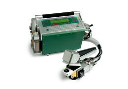
Introduction

Canopy gas exchange systems are useful for quantifying the effects of environmental changes on the instantaneous productivity of a plant community. Measuring the gas exchange of the entire canopy with a chamber system obviates difficulties encountered when extrapolating leaf measurements to the canopy scale such as accurately modeling the distribution of absorbed radiation. Canopy gas exchange systems, if properly designed and operated, can provide a measure of CO₂ flux that closely approximates natural conditions. However, it is important to consider how the chamber may alter, among other factors, the canopy temperature, wind speed (and therefore boundary layer conductance), and radiation balance of the plant community. When possible, canopy chamber results should be compared to micrometeorological flux measurements, since they do not disturb the environment around the canopy (Baldocchi et. al., 1988).

Oftentimes the focus of a study is an individual species of a plant community, or field plots are too small to make use of micrometeorological techniques. In these cases enclosure methods are the only methods available to determine instantaneous canopy CO₂ flux. Many types of chambers and systems have been designed and will not be reviewed here. Garcia et. al. (1990) summarize some of the advantages and disadvantages of open and closed canopy chamber systems.

This application note will be concerned with the design and implementation of a simple continuous flow “open” canopy chamber system based around the LI-6400 Portable Photosynthesis System. This system allows steady-state canopy fluxes to be measured over a period of several hours or days, and is less susceptible to errors introduced by leaks and water sorption than a closed system. (Water sorption can have a significant effect on transpiration estimates until equilibrium conditions are reached.) Nonetheless, depending on plant material and experimental design, a closed system may be more suitable. In that case, the LI-6200 Portable Photosynthesis System may be readily adapted for closed system canopy measurements (Vourlitis et. al., 1993). For soil respiration measurements, the LI-6200 with the 6000-09 Soil Respiration Chamber has been thoroughly tested (Norman et. al., 1992) and is recommended.

Materials and Methods

The LI-6400 system hardware and software flexibility make it a simple procedure to configure it for continuous flow canopy gas exchange measurements. The purpose of this application note is to provide a generic protocol for a wide variety of user-built chambers. Because of the diverse measurement requirements LI-COR does not market a canopy chamber; however some general guidelines for chamber materials and construction, flow measurement, blowers, pumps, external sensors, and a flow schematic are given here to assist you in getting started. A continuous flow canopy chamber was built and tested to prove the concept and to provide an example of how to design and configure the system.

Flow Schematic, System Hardware, and External Sensors

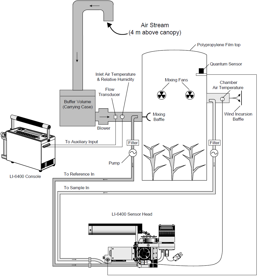
Figure 1 shows the path of air flow through the system and the system components. The system was designed to be portable enough to be moved with reasonable ease from one site to another while operating entirely from 12VDC battery power.

The chamber consists of an extruded cylindrical section of acrylic approximately 45 cm inside diameter (ID), 0.6 cm wall thickness, and 61 cm tall. The top of the chamber is covered with PVdC coated polypropylene (Propafilm®-C, ICI Americas Inc., Wilmington, DE, USA), a transparent film with a high thermal transmittance which helps to moderate temperature increases inside the chamber. The bottom of the chamber is open so that it can be placed over the individual plant or plant canopy. Sufficient air moves through the system so that, due to the flow resistance from the wind incursion baffle at the effluent side of the chamber, a positive pressure is created inside the chamber and leaks are outward.

Air enters a large buffer volume (which also serves as a carrying case for the chamber) through a 5 cm (2 inch) ID rigid PVC plastic pipe that is positioned to pull air from several meters above the canopy. This serves to dampen fluctuations in the incoming CO₂ concentration. A miniature centrifugal blower (TBK-2, Brailsford & Company, Rye, NY, USA) provides about 0.54 m3 min^-1 of flow through the system. It is mounted on the buffer volume. The buffer volume and the chamber are connected by about one meter of flexible tubing and approximately 2 meters of 6.2 cm (2.5 inch) ID schedule 40 PVC plastic pipe. The pipe is painted white to minimize deterioration due to UV radiation. This pipe was selected for its rigidity and size to accommodate the flow measurement.

The chamber volume is approximately 0.094 m3, so the air in the chamber is exchanged more than 5 times per minute. Flow rate may be adjusted by varying the voltage to the blower or by changing the resistance to flow by inserting foam or paper screens inside the wind incursion baffle. As a general rule of thumb the air should be exchanged at least 3 to 4 times per minute through the chamber. A flow transducer (8450-50MV-03-NC, TSI Inc., St. Paul, MN, USA) measures the air velocity just upstream from the chamber. Volumetric flow is computed from the air velocity and the diameter of the pipe and then converted to mole flow rate. Mixing the air to prevent stratification or “dead” air pockets within the chamber is crucial because the sample that is withdrawn from the enclosure must represent the entire volume. Chamber mixing is accomplished by two small axial fans (LI-COR part #6000-17) positioned tangential to the chamber wall and opposite of one another about halfway up the chamber. A cone-shaped perforated mixing baffle is mounted just beyond the point at which the air enters the chamber and supplements the mixing of the mixing fans by distributing the incoming flow to the upper, center, and lower portions of the chamber.

It is possible to quantitatively test the efficiency of mixing and flow measurement accuracy within a flow through system by measuring the time response of the outlet minus the inlet CO₂ differential resulting from continuous injection of pure CO₂ into the chamber (Garcia et al., 1990). The mixing efficiency will vary depending on the canopy height and density, fan type and speed, fan position, and chamber geometry. Air is subsampled just before it enters and just as it exits the chamber by a miniature diaphragm pump with two pumping sections that operate in parallel (TD-4X2NA-Type 4-Viton Elastomers, Brailsford & Co., Rye, NY, USA). Air is pumped to the reference analyzer from the incoming side and to the sample analyzer from the effluent side. The flow rate is approximately 1 liter min^-1 from each side of the pump so that the impact of water sorption and CO₂ diffusion in the Bev-ALine tubing and filters between the chamber and the analyzers is minimized. The air is filtered by two Gelman Acro-50 1 mm filters (LI-COR part #9967-008) before entering the IRGAs.

The inlet air temperature and relative humidity are monitored using a humidity and temperature sensor (Humitter 50Y, Vaisala, Helsinki, Finland) mounted in the chamber inlet air stream. Chamber air temperature is measured with a thermocouple (LI-6400 leaf temperature thermocouple, part #6400-04) positioned in the effluent airstream and connected to the leaf thermocouple input on the LI-6400 sensor head.

This system did not have a means of measuring foliage temperature. Depending on the canopy structure and view angle of an infrared thermometer (IRT), it may be useful to measure the canopy temperature inside the chamber by infrared thermometry (Garcia et al., 1995). Quantum flux density is measured inside the chamber approximately 2 cm below the top with a LI-COR LI-190SA quantum sensor.

Configuring the Software and the Auxiliary Port

In order to operate the flow transducer and external sensors it is necessary to configure the software and auxiliary port to accept and process these signals so that transpiration, assimilation, and other parameters may be computed and recorded in real time.

NOTE: The procedure for configuring the system software requires OPEN version 2.0 or greater, and may vary between different software versions. The description given here is for OPEN software version 2.0.

Follow these 6 steps to set up the software and auxiliary port:

1. Connect the external sensors to the auxiliary port.
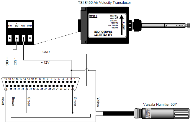
2. Pin assignments for the 37-pin auxiliary port are given in Appendix C of the LI-6400 Primer. The pin numbers are stamped on the connector provided in the spares kit. We have configured the connector to use differential input channels 20, 21, and 22 (Figure 2). The differential ground of the Vaisala sensors is tied to the digital ground because the Vaisala 50Y has no separate ground for signal and power.
2. Add the spare channels to the Configuration File.
3. From the initial startup screen go to the Config Menu and enter the Config Editor. Press Add (f2) and the Master List of configuration options will appear. Scroll to the UserChan= command and press Select (f5). Repeat this process of adding a user channel to the config list 2 more times. You will have three entries that appear as UserChan= 0 0 0. Highlight the first entry and press Edit. Press 0, 5, then L. Your entry will now appear as
4. UserChan= 20 5 0
5. Edit the remaining two channels to look like this:

1. User channels 20 and 21 now are configured for the humidity and temperature sensors, respectively; they use differential ground number 5 (which is tied to the digital ground on pin 20); and the resolution is set to low (0). User channel 22 is configured to measure the flow transducer, using differential ground number 7 with low resolution.
2. Store this as “Canopy Config” by pressing the labels key and then choosing the StoreAs (f5) function key. Press the labels key and then OK (f5) to implement this Config file. For further information about Config files see Technical Note #3.
1. Change the Compute List to accommodate the new calculations.
2. Select User Compute List Editor from the Config Menu. Add the following channels, plus decimal time to the compute list. Assign decimal time to user variable ID 01; humidity and temperature to user variable ID's 91 and 92, respectively; and flow into user variable ID 93. Below is a sample of how the first 5 items in the compute list could be programmed to accomplish this (include all spaces):

3. ##01F5 “Hrs” “Decimal hrs. of OBS Time”

   “$ GETTDS TIME ROT 3600. / SWAP 60. / + +”

   ##91F1 “xRH” “external humidity”

   “chan20_mv * 0.1”

   ##92F2 “xTair” “external temperature”

   “chan21_mv * 0.1 - 40”

   ##93F0 “xFlow” “external flow”

   “chan22_mv * 0.1 * 30.1907 * 44.64”

   ##10 “(U/S)” “flow:area ratio”

   “#93 / area_cm2 / 100.0”

4. “Hrs” will allow us to record the observation time in decimal hours, which is needed to plot data against time. “xRH” and “xTair” are values of external humidity and air temperature, respectively. “xFlow” is the value for air flow through the canopy chamber system. Note that external flow measured from the flow transducer (user variable ID 93) is now used in the flow:area ratio (user variable ID 10), which in turn is used in the transpiration and photosynthesis computations in user variable IDs 20 and 30, respectively.
5. Store this new compute list file by pressing Escape and S to store it with a new file name. Let’s call this new Compute List file “Canopy”. When you Quit the Editor and are asked if you want to implement this new file, type Y for yes. If you would like to add other computations to the “Canopy” file, such as Transpiration Efficiency, the procedure is discussed in LI-6400 Technical Note #2 - Defining Equations for Open.
2. Add the external sensors to the Display file.
3. Since we want to view the status of our sensors in the New Measurements Display, enter New Msmnts from the OPEN screen, and press the Display Editor function key (level 6, f4). Follow these steps to add and store the three new sensors to a display definition:
4. • Press Display Editor (f4).
   • Press Add (f2) to add an additional display line.
   • Use the arrow keys to highlight xRH.
   • Press Select (f5).
   • Select xTair and xFlow, then Escape to quit after adding the three variables.
   • Press OK (f5). When prompted to store the changes, press Y. Name the new Display file “Canopy Displays”, and press Select. When you return to the New Measurements screen, you can put this line on the screen by pressing the letter associated with this new line. The new line will be displayed at the end of the Display Editor list.
3. Edit and store a new LogList file.
4. In order to record data from the external sensors, we must edit the LogList file. While still in New Msmnts, select the Loglist Editor function key (level 5, f5).
5. Add and store the new channels to the LogList file as described below.
6. Use the arrow keys to scroll down until the Insert label appears. Press Insert (f2) to add a variable from the list before the currently highlighted variable. Scroll the list until xRH is highlighted and press Select (f5) or Enter.
7. • Select xTair and xFlow as described above.
   • Press Store and enter "Canopy Output" for the file name.
   • Press OK to implement the new LogList.
4. Store the new Config File.
5. Access the "Canopy Config" file again by selecting Config Editor in the Config Menu. Press labels and then press StoreAs (f5). Name the file "Canopy Config" if it is not already named. It should look similar to the following list (depending, of course, on the optional accessories you may have installed):

6. UserChan= 20 5 0

   UserChan= 21 5 0

   UserChan= 22 7 0

   LightSource= “Sun+Sky” 1.0 0.19

   AREA= 1543 (ground area in cm2 covered by the chamber)

   STOMRAT= 1

   ComputeList= “Canopy”

   Displays= “Canopy Displays”

   StripDefs= “Photo & CV” (or whatever you want this to be)

   LogFormat= “Canopy Output”

7. Now OK this configuration to store your changes and the system software is ready.

Precautions

• Zero and span the LI-6400 IRGAs before measuring. It may be necessary to zero the IRGAs during the measurement sequence: refer to the calibration section of the manual.
• Check the external sensors by blowing on the Humitter sensor; turn the blower on and off to check the flow transducer.
• It may be necessary to match the IRGAs periodically. This can be accomplished in the AutoLog program.
• Do not use the evapotranspiration measured in the chamber to estimate that which is occurring in natural field conditions.
• In well-developed canopies, make sure the chamber is large enough so that edge effects have a minimal impact on the canopy radiation climate.
• The pump in the LI-6400 console is not used for the hardware configuration as described here. However, if you intend to program your system to autolog data and you are using the Match option, then it is currently necessary to leave the pump ON. This is because the automatch routine uses the flow rate through the IRGAs, as measured by the mass flow meter in the console, to determine how long to delay matching after the match valve has been activated. If the console pump is shut off and the console flow meter reads zero, the system will not match.

Alternatively, you can edit the AutoLog program (found in the /User/Configs/AutoProgs directory) by adding a line that reads

right before the line that reads quitAfter NLOOP, and by adding a line that reads

right after the line that reads LPCleanup at the end of the program.

See LI-6400 Technical Note #6 for more discussion on AutoLog routines.

Results

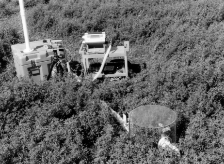
The system as described was installed in a field of alfalfa (Medicago sativa L.) in late August (photo on page 1). The system was programmed to record observations every 2 minutes and to automatically match the analyzers every 5 observations. After the gas exchange measurements were completed the plants which had been enclosed for the measurements were harvested for leaf area determinations. The crop was flowering and had a leaf area index of about 3.7.

There were clear sky conditions on the first full day of measurements (Figure 3), whereas, the second day of measurements could be characterized by scattered cloudy conditions. The canopy CO₂ exchange rates generally followed the diurnal courses of incident light. The maximum air saturation deficits (D) were 3.5 kPa on 25 August and 3.4 kPa on 26 August.

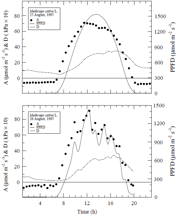
The alfalfa photosynthesis data of 25 August are similar in magnitude and in behavior to those of Baldocchi et. al. (1981). They speculated that the "midday depression" in their data may have been due to starch accumulation in the leaves. Another possibility is that photoinhibition suppressed the rates.

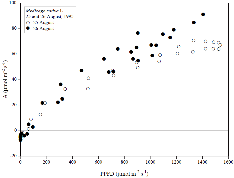
We did not do a time course assay of starch in the leaves; however, a comparison of the photosynthesis data of 25 and 26 August plotted against light (Figure 4) would lend support to either of these hypotheses. In contrast to 25 August, CO₂ exchange rates on 26 August, a scattered cloudy day, did not light saturate.

References

1

Baldocchi, Dennis D., Bruce B. Hicks and Tilden P. Meyers, 1988. Measuring Biosphere-Atmosphere Exchanges of Biologically Related Gases with Micrometeorological Methods. Ecology 69(5), 1331-1340.

2

Baldocchi, Dennis D., Shashi B. Verma and Norman J. Rosenberg, 1981. Seasonal and Diurnal Variation in the CO2 Flux and CO2-Water Flux Ratio of Alfalfa. Ag. Met. 23, 231-244.

3

Garcia, R.L., John M. Norman and Dayle K. McDermitt, 1990. Measurements of Canopy Gas Exchange Using an Open Chamber System. Remote Sensing Reviews, Vol 5(1), 141-162.

4

Norman, J.M., R. Garcia and S.B. Verma, 1992. Soil Surface CO2 Fluxes and the Carbon Budget of a Grassland. J. of Geo. Res. 97, 18845-18853.

5

Vourlitis, G.L., W.C. Oechel, S.J. Hastings and M.A. Jenkins, 1993. A System for Measuring in situ CO2 and CH4 Flux in Unmanaged Ecosystems: An Arctic Example. Functional Ecology 7, 369-379.