Tour #2: New Measurement Mode Basics
New Measurements mode is entered by pressing f4 (New Msmnts) while in OPEN’s main screen. When using the LI-6400, you will likely spend most of your time here, coming out only to do configuration changes, calibrations, lunch, and other ancillary operations.
The New Measurements screen (Figure 3‑10) has three rows of variables with highlighted labels above each. A row of function key labels appears at the bottom.
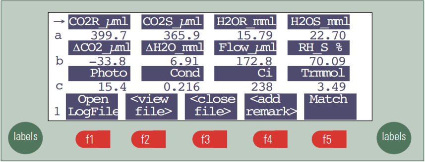
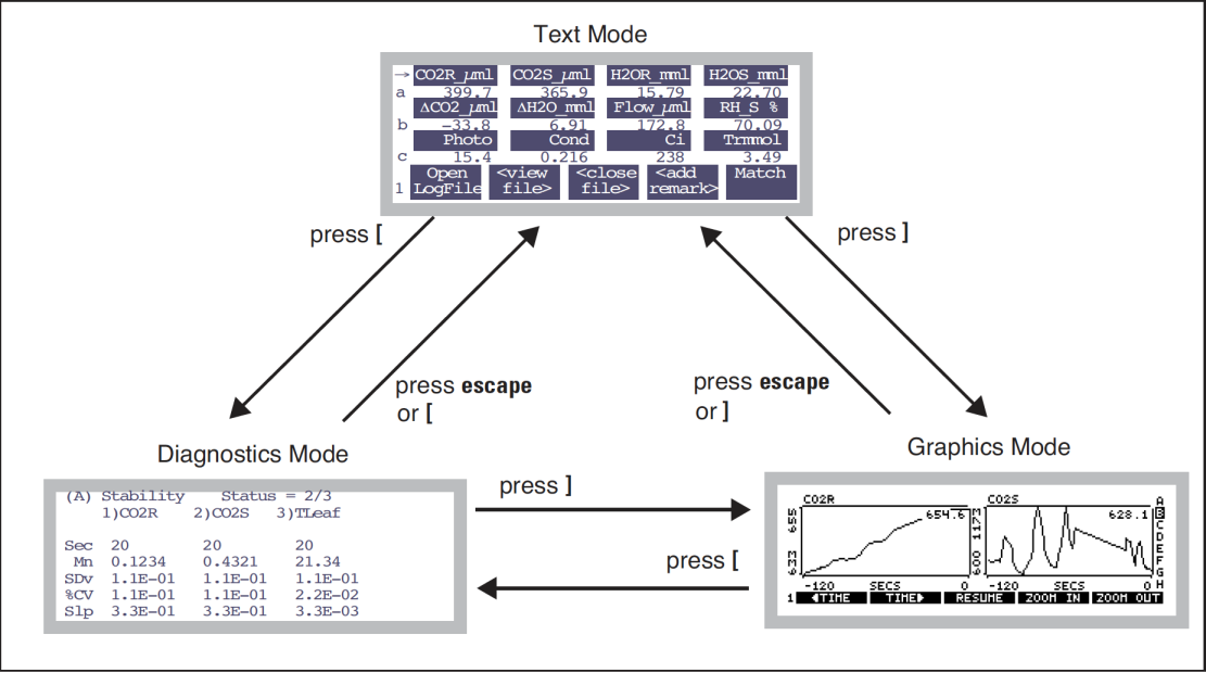
In New Measurements mode, there are two other display modes for providing information. In addition to this text mode, there is Graphics mode and Diagnostics mode. Figure 3‑11 summarizes how to switch between these modes.
We’ll spend the most time discussing text mode, but before we do, however, here’s a quick glimpse of the other two modes:
- Switch to Graphics
- Press ] (the right square bracket key), and you’ll see real time graphs. Press ] again, and you’ll return to the text screen.
- Switch to Diagnostics
- Now press [, and you’ll enter the diagnostics mode. Press [ again, and you’ll return to the text screen. We’ll be visiting graphics and diagnostics again in our tours in this chapter, and will cover more details then. The "reference section" for all three display modes is in Chapter 6.
Function Keys
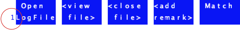
Text mode has 7 sets of function key definitions (or 10 with the Leaf Chamber Fluorometer). The current function key level number is displayed in the bottom left hand corner of the display. If you press labels seven times, you’ll see them all. Here is a shortcut: press the number keys (1 through 7 on the keypad), and you’ll jump directly to that function key level.
To change function key levels:
- Press 1 through 7…
- This directly accesses the selected level.
- …or, press labels or shift labels.
- labels takes you ahead a level, and shift labels takes you back a level.
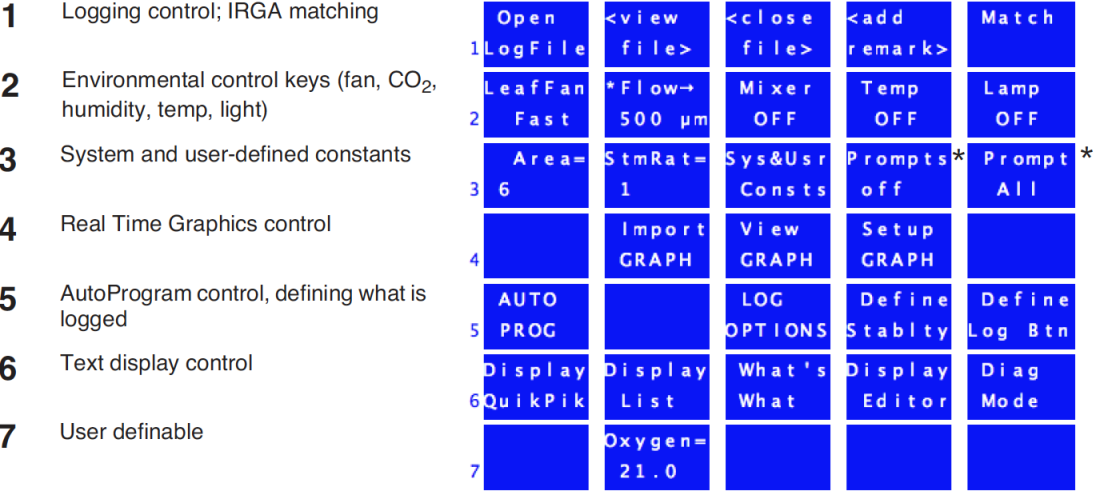
The labels are summarized in Figure 3‑12. Note that the level 7 key labels are all blank in the default configuration, and are available for your own use (described in Example: Using New Measurement’s Fct Keys on page 26-16).
Example: Changing the chamber fan speed
- Access the chamber fan control function key
- Press 2. The function key labels will change as shown in Figure 3‑13.
- Access the control display
- Press f1. The fan speed control box will pop up on the display.
-
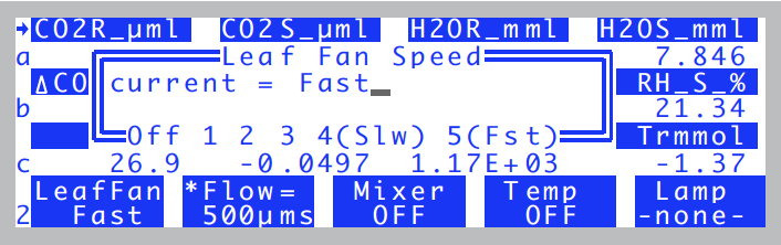
Figure 3‑13. Controlling the fan speed. Press F, S, or O for fast, slow, or off, or 1 thru 5. - Turn the fan off
- Press O (the letter, or the number 0 - both happen to do the same thing here), and the fan will stop. If you listen, you should hear a drop in the noise level, especially if the chamber is open.
- Turn the fan back on (fast)
- Press f1, then f, and the fan will resume running. This is the speed you should normally use. However, a reduced fan speed is helpful for keeping the surface humidity of the leaf high, which can prevent stomatal closure in stressed plants during measurement.
Text Display
Twelve variables are displayed in Figure 3-10 on page 3-15, but there are many more available. Here’s how you display them:
To change a display line:
- Use ▲ or ▼ to select a line
- To the left of each label value line is a letter, and to the left of one label line is an arrow (►). The ► indicates the “change line”. You can select the change line by pressing the ▲ or ▼ keys.
- Press a letter
- Up to 26 display lines can be defined (this corresponds to keys A through Z), although the default display defines only a through l. For example, put the ► marker on the bottom line, and press A. The display will change as shown in Figure 3‑14.
-
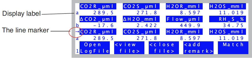
Figure 3‑14. To change a display line, position the marker using ▲ or ▼, then press a letter key. In this figure, we’ve put the marker on the bottom line and pressed A.
- Alternatively, press ◄ or ►
- Pressing the horizontal arrow keys will scroll the change line through all the possible displays, but it is faster to use the letter shortcuts.
- Go exploring!
- Table 3‑2 lists the default displays, and their variables. Use the arrow keys and letter keys to view them yourself. Note that these display definitions can be modified (what variables are shown, and where) to suit nearly any taste. It’s all explained in Chapter 6.
Display Groups
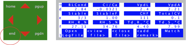
You can change all three lines of the text display with a single keystroke. There are 4 keys reserved to do this: home, pgup, pgdn, and end.
To define (or redefine) a display group, get the display arranged the way you want it, then hold the ctrl key down and press the group key (home, pgup, pgdn, or end) of your choice. That group key is now defined. Once a group key is defined, you can change all three display lines to that arrangement simply by pressing the group key.
Example
Make the home key display lines a, b, and c, and the pgup key display lines g, h, and k.
- Define home key
- Put lines a, b, and c on the display, and press ctrl + home.
- Define pgup key
- Put lines g, h, and k on the display, and press ctrl + pgup.
- Switch displays
- To view a, b, and c, press home. To view g, h, and k, press pgup. You’ve seen how to define the group keys "on the fly". Actually, the display arrangement (what’s in groups a through z) as well as the group key definitions are all user-definable, either through the level 6 function keys in New Measurements mode (Display Editor on page 6-6 in the instruction manual), or editing the
<open> <display> <text>node of the configuration tree.
Real Time Graphics Displays
New Measurements mode also provides a method to monitor these variables graphically. To access the graphics displays, press 4, then f3 (View Graphs). (There is also a short cut: ] the right square bracket key.) The display should show something like Figure 3‑16.
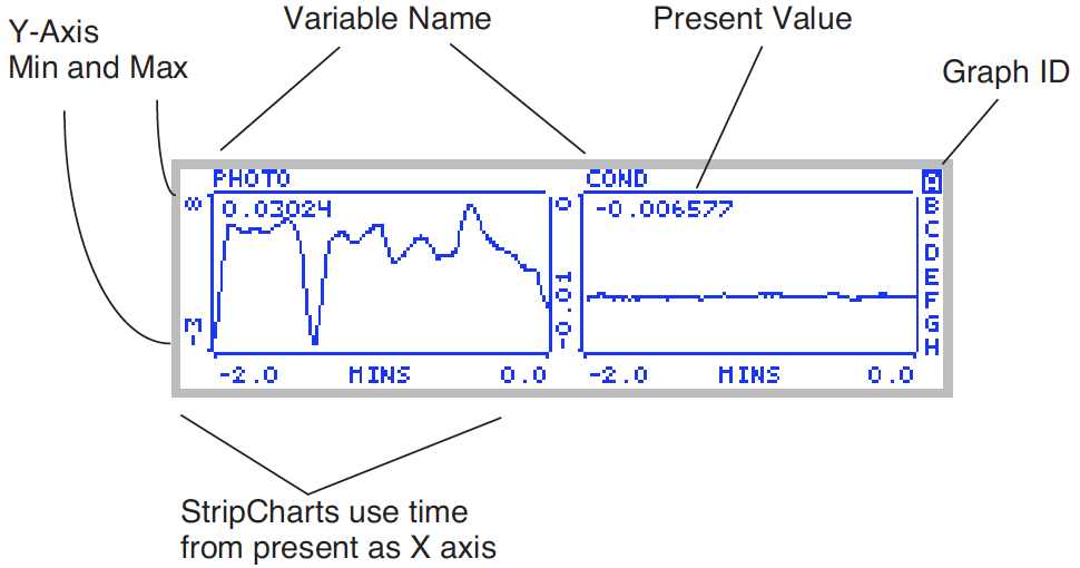
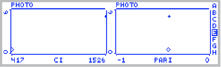
There are 8 RTG displays available in New Measurements mode, and they are designated by the letters A through H. Figure 3‑16 shows the A display. Each display can have 1, 2, or 3 plots. Each plot can be a StripChart - a variable plotted against time with a continuous line, or an XYChart (Figure 3‑17) - one variable plotted against another using discrete points, usually representing logged observations.
Here are two navigational rules:
- To change RTG Displays
- Press the letters A through H to jump directly to a particular display. You can also use the arrow keys ▲ or ▼ to step through them sequentially. The indicator at the right side of each graph will show which graph you are viewing.
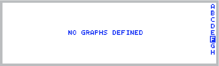
- If no plots are defined for a particular graphics display, it will appear as in Figure 3‑18.
- To exit Graphics Mode
- Press escape or ] to leave graphics mode and go back to the text displays we were looking at earlier.
Graphics Function Keys
There are three levels of function keys associated with New Measurement’s graphics displays. Activate them by pressing labels. The plots shrink a bit to make room for the labels.
Graphics Function Key Tour
Let’s try out some of the function keys. Find a graphics display that has strip charts on it, and press labels to bring up the labels.
- Note that labels are an attribute of each graph
- The function key labels for each graphics display are independent. Change to another display, and the labels go away. That is, turning them on for one graph, doesn’t turn them on for any other.
- There are 3 levels of function keys
- You can navigate them just like in text mode: press labels, or press 1, 2, or 3. You can also use this shortcut to bring up the labels. When real time graphics labels are not visible, the function keys are not operative.
- Turn off the labels
- Press the HIDEKEYS key (f5 level 2), and the labels disappear. Another way to turn off the labels is to press the number 0.
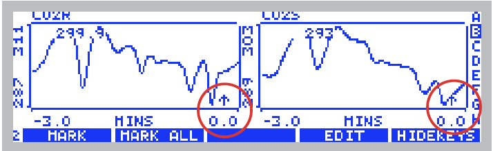
- Mark the graphs
- Press MARK (f1 level 2), and a small arrow (↑) will appear on each StripChart on this display.
- As you might expect, MARK ALL marks all of the displays (A - H). Plots are marked with a small ’+’. These marks also happen automatically to all graphs when you log data (a topic that lies ahead of us).
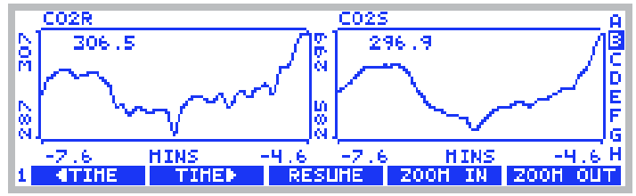
- Travel back in time
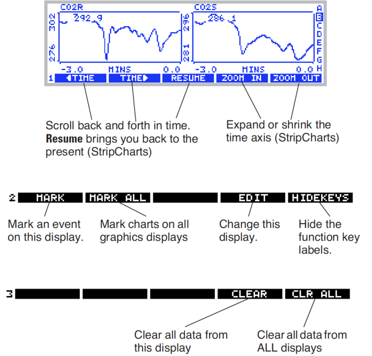
- Our StripCharts in Figure 3‑21 are showing 120 seconds of activity, but they remember more than that (10 minutes by default, but it’s user definable). Press 1 to access the time control function keys, and press f1(◄TIME) several times (Figure 3‑21). Note that the time axis continues to show 2 minutes worth of data, but at earlier and earlier times. Note too that the plots stop updating while we scroll back, although data continues to be collected and saved. The axis time labels still reflect time since the present.
- To resume normal plotting, you can press f3 (RESUME), or scroll back to the present with f2 (TIME►), or simply wait for about 15 seconds, in which case plotting automatically resumes.
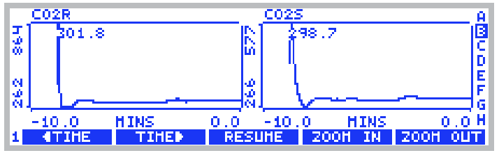
- Zoom in, Zoom out
- The remaining two time control keys, ZOOM IN and ZOOM OUT, change the range of the time axis on StripCharts. Thus, if you wish to see the big picture, start pressing f5 (ZOOM OUT) (Figure 3‑22).
- Now, press ZOOM IN several times to return to 2 minute display width.
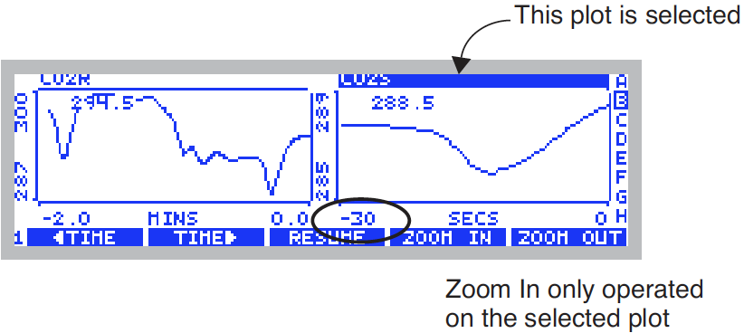
- Selecting a Chart
- Normally, the time control keys operate on all of the StripCharts in the display being viewed. (They do nothing to XYCharts). You can, however, select an individual chart by pressing the left or right arrows (◄ ►). An inverse bar appears over the selected plot (Figure 3‑23). Now, pressing a time control key will operate on only that plot.
- Exit graphics mode
- There are two ways back to normal text mode: escape or ]. Note that the ] key brings you into graphics mode, and also takes you out.