Stability Considerations
In New Measurements mode, the LI-6400 measures and computes continually, regardless of the state of equilibrium of the leaf in the chamber. It can also log data with the same disregard for stability. The question is, how do you know when the system is stable enough to record meaningful data? Also, when you log an observation, how can you tell, when you look at the data later, how stable the reading was?
Stability Indicators
Version 5 introduces a powerful technique for determining system stability (Stability Indicators on page 6-29 in the instruction manual). It allows you to set up criteria based on measured and computed variables, to determine when the system is stable. For each variable chosen, stability can be based on statistics (any combination of standard deviation, rate of change, and coefficient of variation) over a time period of your choosing. Table 4‑1 indicates a typical definition.
| Variable | Time (s) | Standard Deviation | Coefficient of Variation (%) | Rate of Change (per minute) |
|---|---|---|---|---|
| PHOTO | 20 | < 0.5 | < 0.1 | |
| COND | 20 | < 0.1 | < 0.05 |
The shaded entries are “don’t care”. That is, they don’t enter into the decision. Therefore, with the definition given in Table 4‑1, if one or more of the nonshaded conditions is not met, the system would be considered unstable.
What variables should be checked?
There are two approaches to determining system stability: Check all the inputs, or check the results. By inputs, we mean the list of variables that go into calculating photosynthesis and conductance: CO2R, CO2S, H2OR, H2OS, Flow, Tleaf. Add to that list ParIn, since light is driving photosynthesis. If all of those were stable, then certainly PHOTO and COND will be stable.
The merit of checking just the results, PHOTO and COND, is that it is simple. On the other hand, keeping statistics on all of the inputs is good for diagnostic purposes. For example, if PHOTO is not stable, why is it that way? Is the flow rate varying (automatic humidity control)? Is CO2R unstable? If CO2R is stable, but CO2S is not, it could be resulting from flow fluctuations, or from ParIn fluctuations. And so on.
What statistics should be checked?
At first glance, time rate of change seems sufficient. If that’s all you check, you could run the risk of calling a signal stable that was noisy or in transition, and just happened to have a rate of change (slope of a straight line fitted to values of the signal plotted against time), near zero at one instant in time. If you were only considering one variable in the stability definition, then just looking at only the rate of change could be risky. If you have several variables included, then the chances of getting fooled go down.
Logging Stability Indicators
The Log Options part of the configuration includes something that provides information on system stability at the time of logging (Figure 4‑9).
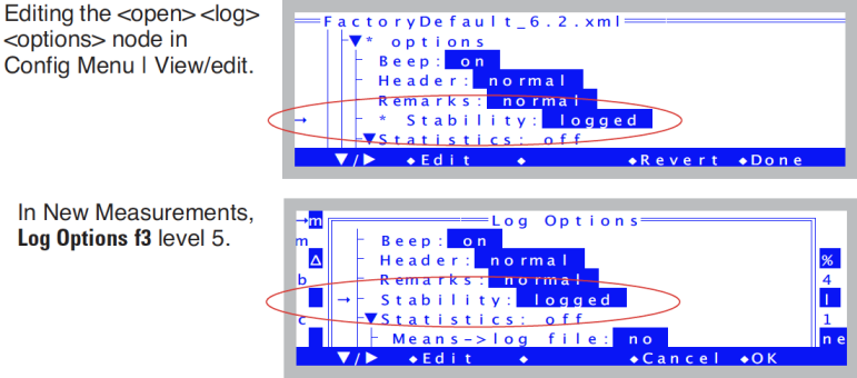
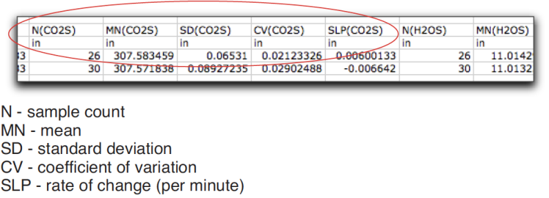
The stability entry can be “no” or “logged”. When it is set to “logged”, there will be 5 extra columns in your data file for each variable that you have in your stability criteria (Figure 4‑10).
Real Time Graphics
A useful visual indicator of stability can be had with judicious use of New Measurement’s strip chart mode (Real Time Graphics on page 6-14 in the instruction manual). You can plot photosynthesis and conductance as a function of time, and watch for any trends over the past minute or two, or more.
If you are using a buffer volume, it is useful to keep an ongoing plot of reference CO2, so that if photosynthesis doesn’t seem to be stabilizing, you can quickly tell if the problem is physiology (reference is stable) or mechanical (reference is unstable).
Average Time
You have at your disposal a configuration parameter that influences stability. It is the <open> <a2d> <avgtime> node in the configuration tree (Averaging Time on page 16-22 in the instruction manual). By default, it is 4 seconds, but you can raise or lower that number if you wish.
If you require the quietest possible signal, and can afford longer equilibrium times, then you may want to raise this number to 10 or 15 seconds. If, however, you are trying to measure transients, or the system dynamics need to be optimized, then set this to 0.5. (Any value at or below 0.5 will give you 0.5 second averaging, which is the frequency of new measurements.) The price will be slightly greater IRGA noise than you’d get at 4 seconds.