Using the 9968-338 sample adapter kit with the 6800-18 aquatic chamber
The aquatic chamber sample adapter kit replaces the viewing window on the 6800-18 aquatic chamber with an easily removable O-ring sealed plug. The plug includes hooks intended to accommodate a wide range of discrete sample geometries, such that these samples can be easily inserted and removed from the chamber and can be held in a fixed position relative to the fluorometer light source. The adapter kit can be used for a range of sample types that may be measured submerged in a liquid media (such as macroalgae, coral, aquatic invertebrates, and others) and water saturated samples measured in humid air (like many bryophytes), that would otherwise be impossible to insert into the aquatic chamber through the sample port normally used for liquid suspensions.
Sample loading consideration
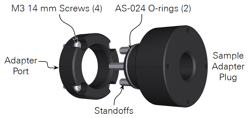
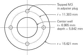
The kit includes a port that replaces the viewing window, allowing direct access to the sample cell of the aquatic chamber, and an adapter plug that serves to seal the chamber and hold the sample during measurements. The kit also includes four 14 mm long stainless-steel standoffs that can be threaded (M3) into the plug and used to hold the sample in a fixed position (spacing for the standoffs is given in Figure 1‑1). Alternatively, a well in the center of the plug can be used to hold the sample directly and is sized to accommodate a nominally 12.5 mm diameter object. A corresponding bore on the dry side of the plug allows for a similarly sized object to be inserted there. An example use case could be, for samples affixed to 12.5 mm diameter plastic coated magnets, an iron rod can be inserted on the dry side making for a magnetic sample mount in the adapter plug.
For samples that will be measured in solution, the sample is typically mounted to the adapter plug and inserted into the chamber “dry”. Then the chamber is filled with the measurement solution through the fill port at the top of the chamber using the syringe and dispensing needle included with the aquatic chamber. Typical measurement volumes for the aquatic chamber are around 15 mL, and with the adapter plug this total volume should be used (liquid plus sample volume). However, unlike measurements of microalgae suspensions, slight over filling of the chamber does not pose a big issue, since ideally the plug keeps all biological material in the illuminated region of the sample cell. Significantly over filling the chamber, however, is still dangerous as it has the potential to force liquid into regions of the measurement system where it should never go. Try to keep the liquid level with a sample in the chamber at or below the channel connecting the sample cell to the sample chamber headspace (upper part of the chamber immediately bellow the fill port).
| Description | Quantity | Part number |
|---|---|---|
| Sample adapter plug | 1 | 6568-685 |
| Sample adapter port | 1 | 6568-684 |
| AS-024 O-ring | 2 | 192-02553 |
| M3 4.5 x 14 mm stainless-steel standoffs | 4 | 161-18848 |
| M3 14 mm pan head screws | 4 | 150-15694 |
Installation
The adapter consists of a mounting ring and an insert that holds the sample. To install it:
- Remove the viewing window on the exposed side of the aquatic chamber.
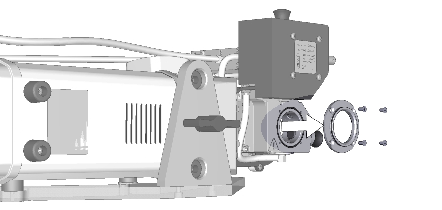
- Install the sample port in its place.
- Be sure the O-ring stays seated in the chamber, then tighten the four screws (150-15694) to secure the port in place.
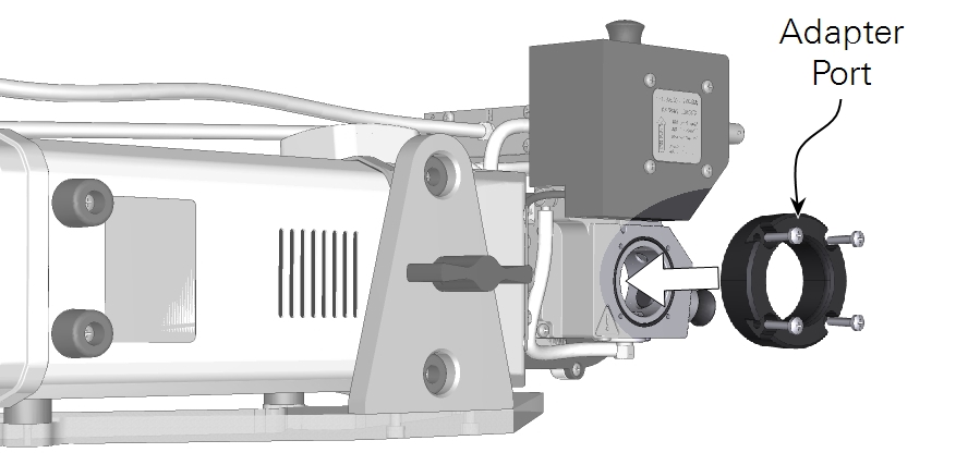
- Load a sample into the chamber using whichever method works best for you. Options include:
- Mount a leaflet using standoffs and O-rings as shown in Figure 1‑3.
- Place a sample directly in the well or secure it as described in Sample loading consideration.
- Press the sample adapter plug firmly into the port.
Standardizing the reported fluxes
The aquatic chamber configuration provides four different carbon dioxide assimilation values, three of which are standardized to some scalar (cell, chlorophyll or mass density) and one unscaled flux velocity (flux per sample). When working with the sample chamber adapter, the three scalar standardized parameters are likely not meaningful. Here, it is probably more useful to report an assimilation standardized by either surface area or sample mass. This can be done simply by dividing the flux velocity (flux reported in μmol s-1) by the desired scalar.
Estimating light incident on the sample
The aquatic chamber has an attachment for placing a LI-COR LI-190R Quantum Sensor on the viewing window normally installed on the chamber. For measurements of uniform sample suspensions (micro algae) this is used to measure how much light is transmitted through the sample, which is in turn used to estimate the absorbed quanta and the mean light intensity in the sample. These parameters, among others, are reported in the AquaticQ data group on the instrument.
However, for discrete samples mounted in a fixed position relative to the light source, as would typically be the case when using the aquatic chamber sample adapter, many of the AquaticQ parameters are not meaningful. This is because either their assumptions are not met in this configuration, or because the sample adapter precludes the real time measurement of light exiting the chamber. Regardless, the normal viewing window and quantum sensor can still be used to make a measurement of chamber transmittance, which can later be used to make an estimate of light incident on the sample in subsequent measurements made with the sample adapter in place.
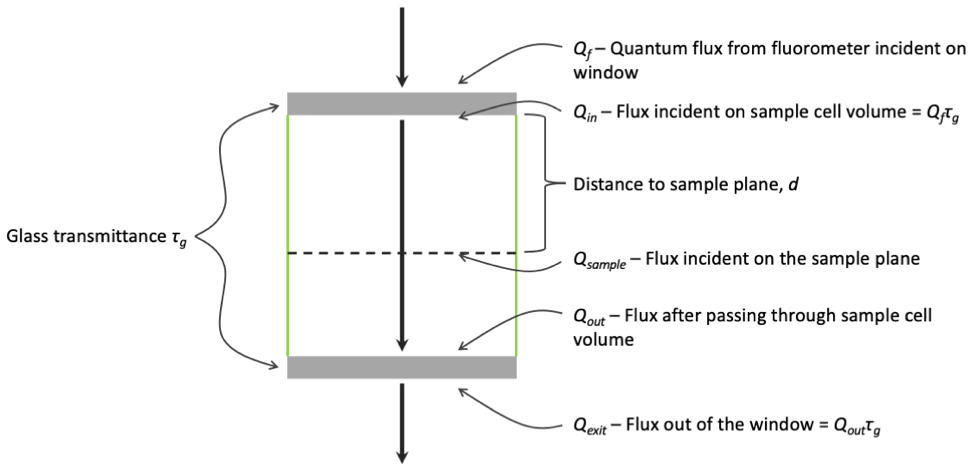
Qf is the flux of photons (μmol m-2 s-1) from the fluorometer incident on the window of the sample cell (Figure 1‑2), and Qexit is the flux leaving the opposite window (when present). The windows (when clean) each have a transmittance, τg, of 0.98. For a sample held at some distance from the fluorometer window (dashed line in Figure 1‑2), the light reaching it, Qsample, will fall somewhere between Qf and Qexit dependent on the optical properties of the sample cell and the measurement solution.
What are the "knowns"? On the fluorometer side, we know Qf, what the fluorometer is generating. If τg is specified, then we actually have Qin reported directly, since the fluorometer takes transmittance into account when setting light levels.
There is a subtlety here: The fluorometer is calibrated with a 6 cm2 aperture, but when used with the aquatic chamber, the aperture is 7.92 cm2. If the fluorometer's light output were perfectly uniform, then increased area would not change the irradiance, since it is on a per area basis. However, the light output is brightest near the edges, and the area increase results in about 20% more light output than expected. This is accounted for in the transmittance factor of 1.18 that is applied when using the aquatic chamber, which includes the window transmittance of 0.98. For example, if you set the fluorometer to 1000 μmol m-2 s-1, it will actually set itself to 1000/1.18 = 847 (according to its 6 cm2 based calibration). The actual output is some 20% higher (1020), which reduces to the 1000 you asked for when it passes through the window into the aquatic chamber.
This slight non-uniformity also matters when positioning the sample with the sample adapter. Where the sample will fill the bulk of the aperture, placing the sample close to fluorometer window means that there will be a light gradient across the sample. For a small sample close to the fluorometer, only filling the center of the aperture, light will be more uniform across it, but the actual intensity incident on the sample will be lower than reported. The non-uniformity across the aperture decreases the further from the fluorometer window the sample is placed, simply due to scattering and internal reflections in the cell. Such that a sample positioned some distance back from the fluorometer window is generally recommended.
With the viewing window and quantum sensor installed, from the quantum sensor reading q we can estimate Qexit. To do this, we must account for calibration differences (due to light spectra, field of view, etc.) between the fluorometer and the particular sensor being used. This difference depends on color (red and blue fractions fr and fb), so we use an empirically determined adjustment factor for each, ar and ab. These are measured using a dry, empty aquatic chamber with the procedure described in the user manual. It is assumed we know the effective transmittance of light through a dry, empty chamber. This has been measured using a fluorometer and an integrating sphere to collect the light. For red, the value is 0.54, and for blue, it is 0.51.
Once ar and ab are known, we can now get Qexit and Qout from q:
1‑1

1‑2

The cell transmittance (τ) is computed from
1‑3

If the sample cell were a perfect "light pipe", the transmittance would be 1.0 when the cell is empty. In reality, it is closer to 0.5, because of light losses to interior surfaces; filling the sample cell with clear water actually increases the transmittance slightly. Since what is of interest here are typically measurements in solution, we can use an empirically determined “clear water” (or culture media, as the case may be) transmittance (τw), as a reference.
With clean water (or whatever solution will be used for measurements) in the sample cell, we define an expression for “clear water” transmittance τw:
1‑4

Since red and blue are scattered slightly differently in the cell, the determination of τw should actually be done twice: once for red light (fr = 1) yielding τwr, and once for blue (fb = 1), yielding τwb. Typical values are τwr = 0.58 and τwb= 0.57. Then, for any mix of fr and fb, the appropriate color-weighted water transmittance τwis:
1‑5

Given this transmittance, we can compute an extinction coefficient (εw) for the “water” filled sample cell. To do this we assume light extinction in the sample cell is a Beer's law process.
1‑6

The value 25.4 here represents the distance in mm between the interior surfaces of the windows across the sample cell.
From the extinction coefficient and Qin, light incident on a plane at some distance, d, from the fluorometer window can be estimated.
1‑7

At the face plane of the sample adapter plug, d is 23.62 mm (25.4 minus 1.78 due to the slight protrusion of the plug into the chamber) and would be 9.62 mm at the top of the standoffs (if used).
In practice, τw, and subsequently εw, should be characterized for a clean chamber with the normal viewing window and quantum sensor installed, filled with whatever solution measurements will be carried out in, and following the procedures outlined in the user manual. Once εw is known, it can be used to compute Qsample for measurements made with the sample adapter in place, in the absence of subsequent measurements with the external quantum sensor.
It should be noted that we have neglected the effect of the pump and resulting bubbles in the analysis up to now, but bubbles may have a significant effect. Typically, they reduce measured qvalues by a factor of 0.7 to 0.8. Correcting for this effect may or may not be important when estimating Qsample using the sample adapter, however. This will depend entirely on the position of the sample plane inside the cell.
To handle the bubble effect, in the standard use of the aquatic chamber (a uniform suspension filling the sample cell volume), we introduce the empirical constant B, which is simply
1‑8

Where qon is the external quantum sensor reading with the circulation pump on, and qoff when it is off.
B is then typically applied when computing the effective clear water transmittance, which is then corrected for color and bubble effect:
1‑9

However, this implementation to correct for the bubble effect poses some potential issues when estimating Qsample with the sample adapter. In effect, it assumes that B is constant across the sample cell, which cannot be not true because the perforations where the bubbles are introduced to the sample cell do not span the full width of the cell. Rather, bubbles are introduced in a band centered at the mid-plane of the cell with a roughly 8 mm wide bubble free zone on either side. This implementation of B is thus only reasonable when the sample is positioned with the full bubble curtain between it and the fluorometer window. If the sample is placed between the bubble curtain and the fluorometer window, Bshould be ignored entirely (B = 1). In any case where the sample is positioned inside the bubble curtain, this implementation of B will introduce some, potentially significant, artifact to the calculation of Qsample.
Some comments on material choices
Where additional parts will be added to the sample adapter plug to accommodate some particular sample material, the user should be mindful of material choices. It is recommended to use a high-quality stainless steel for any metal parts. This material has both good corrosion resistance and no appreciable interaction with carbon dioxide. Unlike other places in the LI-6800, nickel plated aluminum should be avoided for wetted applications. Thin plating, particularly on edges, can lead to rapid corrosion of the underlying substrate for submerged parts, through a nickel catalyzed process that consumes carbon dioxide.
The adapter itself is machined from black acetal. This material works well in wetted gas exchange applications and for fluorometry, as it has no appreciable interaction with carbon dioxide and it does not exhibit auto-fluorescence. For any user added plastic parts, it would be the recommended material. Where other plastics will be used with the adapter, they should be evaluated for auto-fluorescence. We have found that many plastics, particularly those pigmented white, exhibit some degree of auto-fluorescence detectable the 6800-01A. This auto-fluorescence tends to be non-variable in nature and as such generally appears as a consistent bias on the raw fluorescence signals. Depending on the specific parameter being measured this may or may not matter, and best practice would be to simply avoid these materials.
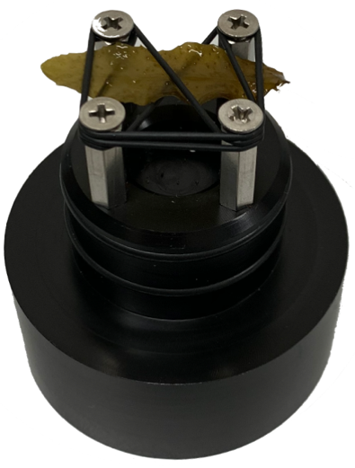
A measurement example using the macroalgae Sargassum
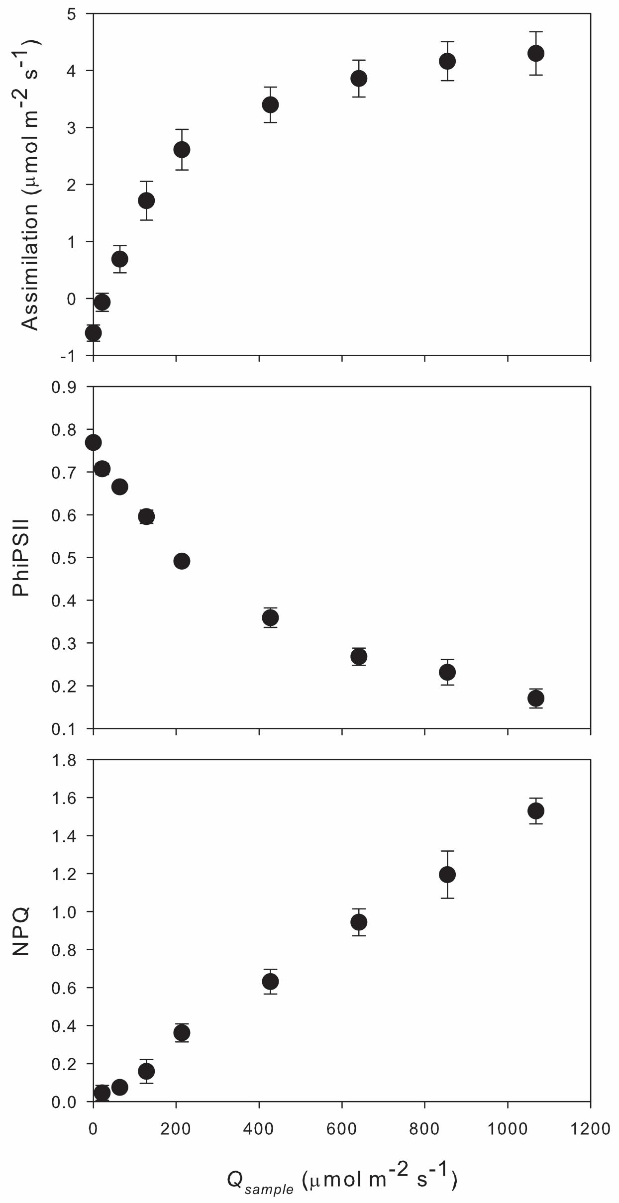
Here we show an example data set where the sample adapter plug was configured to hold a leaf-like sample. This arrangement requires four additional screws and two O-rings (user-supplied or retrieved from the instrument spares kit). The 14 mm standoffs were attached to the plug with flat head screws threaded into their open ends, providing a small lip at the end of the standoff. Two Viton rubber O-rings were then wound between the standoffs under this lip, such that a small flat sample could be held between them (Figure 1‑3), at a position where bubbles in the chamber were predominantly on the unilluminated side of the sample. Measurements of photosynthetic response to irradiance (Figure 1‑4) were made starting from darkness on three replicate samples of Sargassum. Assimilation rates were standardized by projected surface area of the sample (average of 2.26 cm2), and Qsample was calculated using d=8.5 mm. Transmittance was determined with the pump off and the extinction coefficient was calculated for the 50:50 red:blue light mix used for measurements (τw =0.625=0.64*0.5+0.61*0.5, εw =0.0185=-ln0.625/25.4). Measurements were made in synthetic seawater.