Response curve Background Programs

In principal, generating a response curve consists of the following repetitive pattern: 1) set environmental conditions, 2) wait for stability, 3) log data.

BPs provide a fair amount of flexibility for accomplishing these tasks: Control setpoints can be hand-entered, read from a file, generated from an algorithm, and so on. Wait times can be fixed, or made to adapt to conditions.

The following sections illustrate some response curve options available with BPs.

Basic

A simple BP to generate a response curve for CO2 can be found in the Library GROUPS source, and is shown in Figure 12‑45. To change setpoints, edit the LOOP step, and to change target, edit the SETCONTROL step.

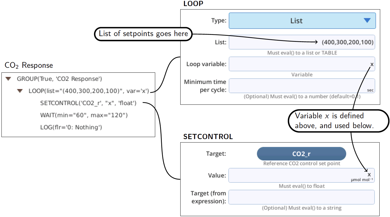
Since the list entry in LOOP is evaluated, you can use Python expressions there. For example, if you wanted integer setpoints every 100 ppm from 100 to 1000, you could make use of the range() method, which takes integer arguments of start, stop, and step.

which would (at run time) make the list

Another option is shown in Figure 12‑46, where we've added an EXEC step to make available some list generating utility methods available in the module list utility.py). We use that capability to generate a floating point setpoint list given simply a start value, stop value, and number of desired points.

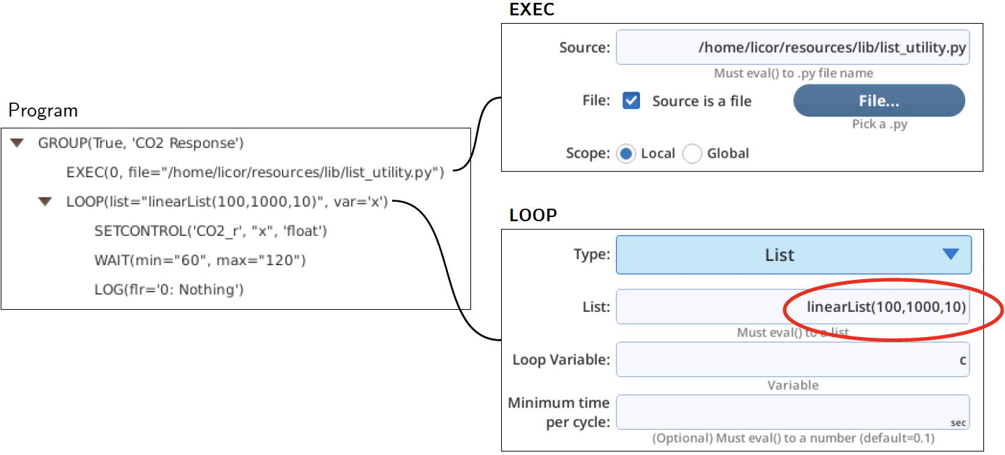
If you want randomized values, use randomList() instead of linearList().

Table 12‑1. Examples of randomList(), and linearList().

Expression	Result
linearList(1,10,4)	[1.0, 4.0, 7.0, 10.0]
linearList(5, -5, 6)	[5.0, 3.0, 1.0, -3.0, -5.0]
randomList(5, -5, 11)	[4.0, 3.0, -1.0, -3.0, 2.0, 1.0, -2.0, -4.0, -5.0, 0.0, 5.0]

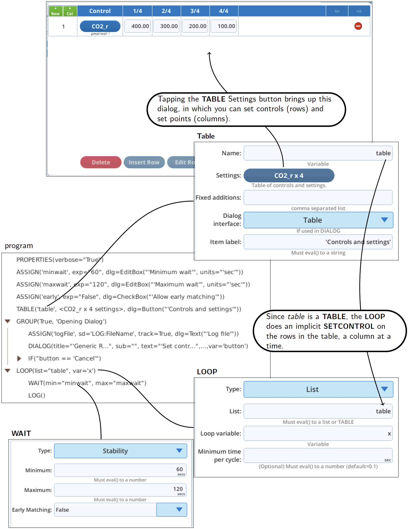
The sample program /home/licor/apps/basic/GenericResponse.py (Figure 12‑47) illustrates the use of a TABLE, which makes it easy to coordinate targets and setpoints. Table entries do not by default pass through eval() (i.e., no expressions, no variables), so setpoints have to be explicitly entered.

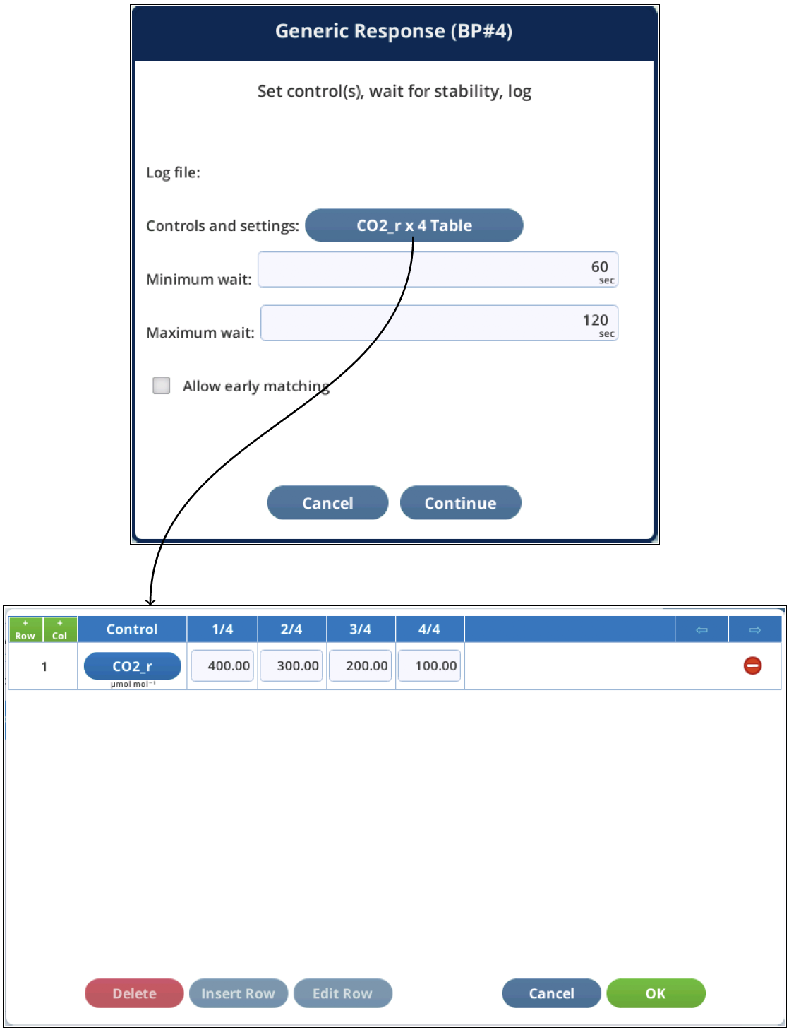
The GenericResponse.py program does support an opening dialog (Figure 12‑48), from which you can also edit the table.

Multiple controls

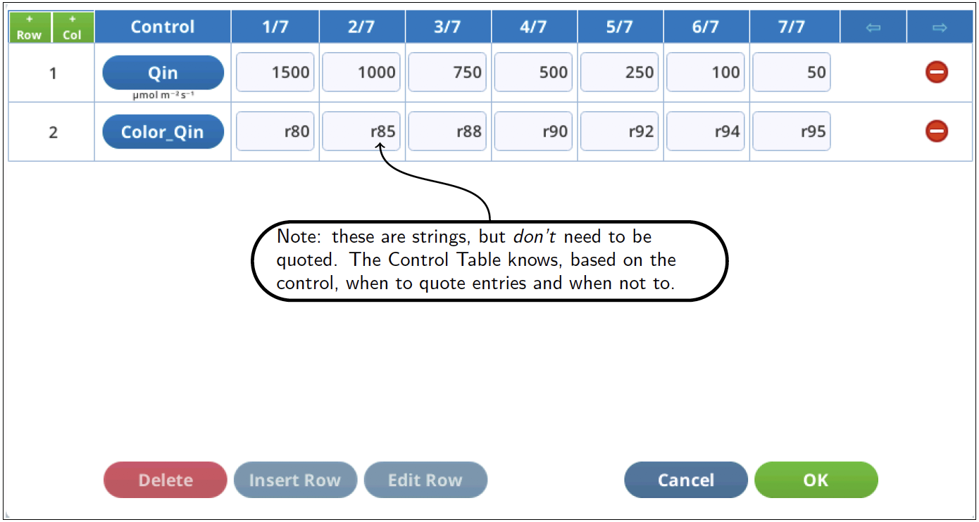
How to change multiple controls in a response loop? For example, how could you make a light response with the color becoming more red as intensity drops?

One method is to use the control table interface (such as with /home/licor/apps/basic/GenericResponse.py), and make the table look something like this (Figure 12‑49):

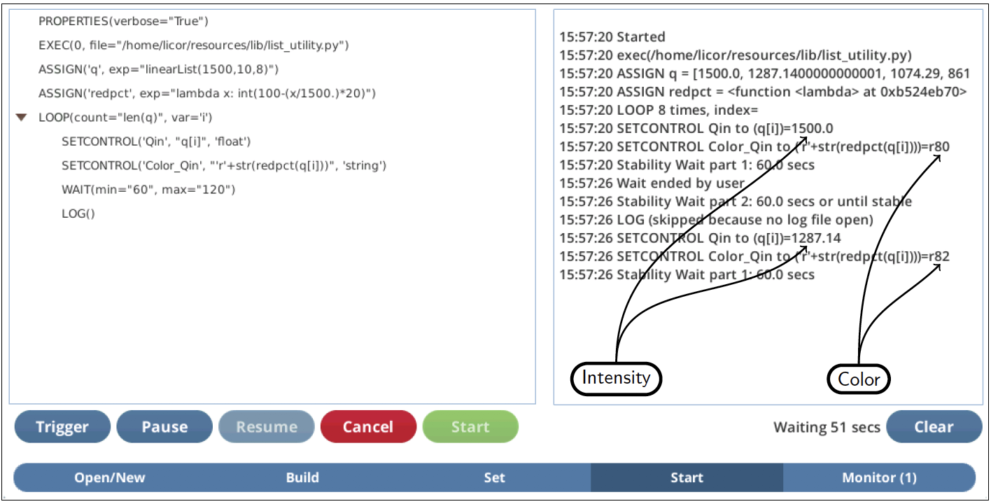
Another method is illustrated by the example program /home/licor/apps/examples/LightColorCurve.py (Figure 12‑50), which uses programmatically determined setpoints for intensity and color.

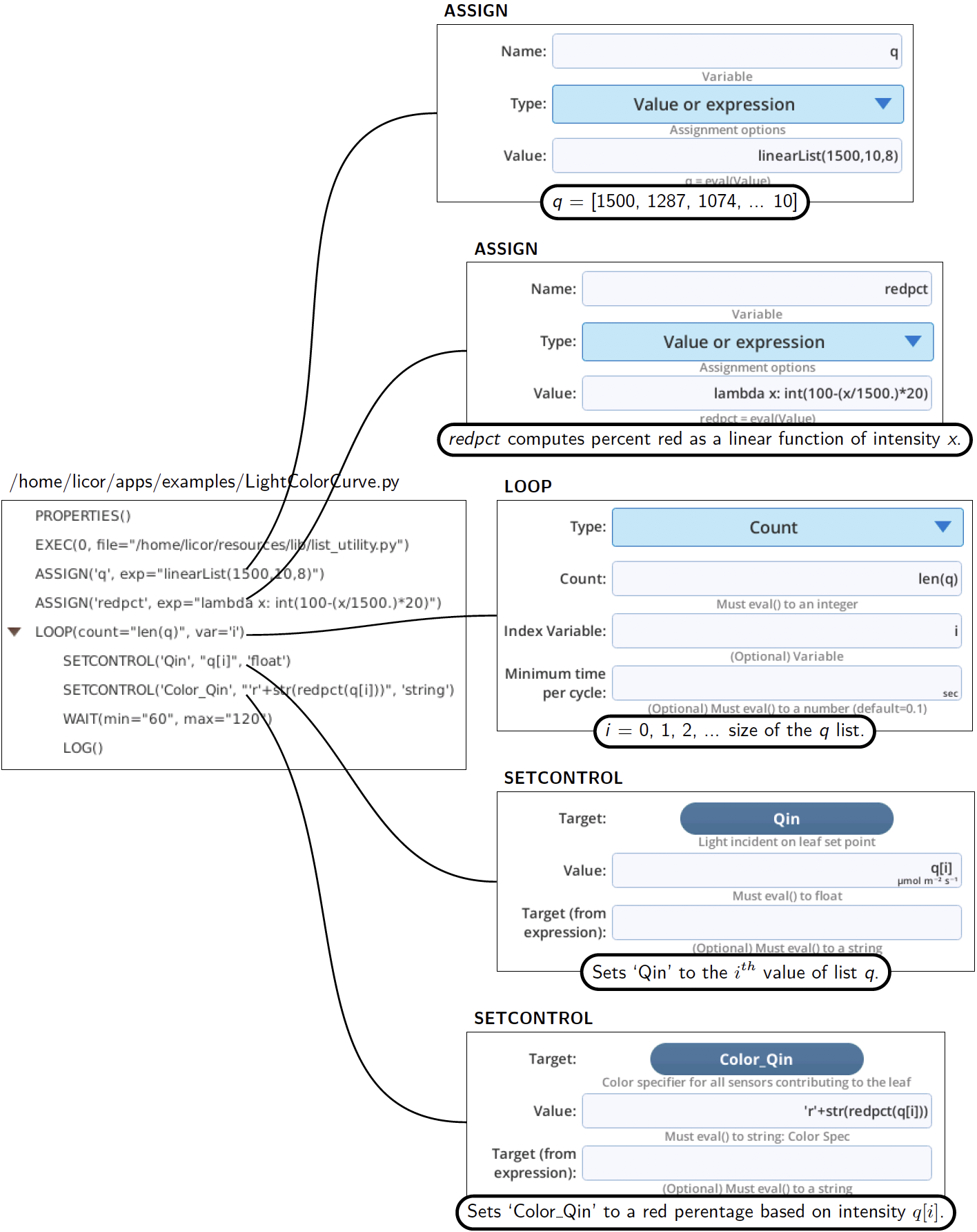
If we test run this program in verbose mode, we can see the values it picks for the each setpoint (Figure 12‑51).

Higher dimensions

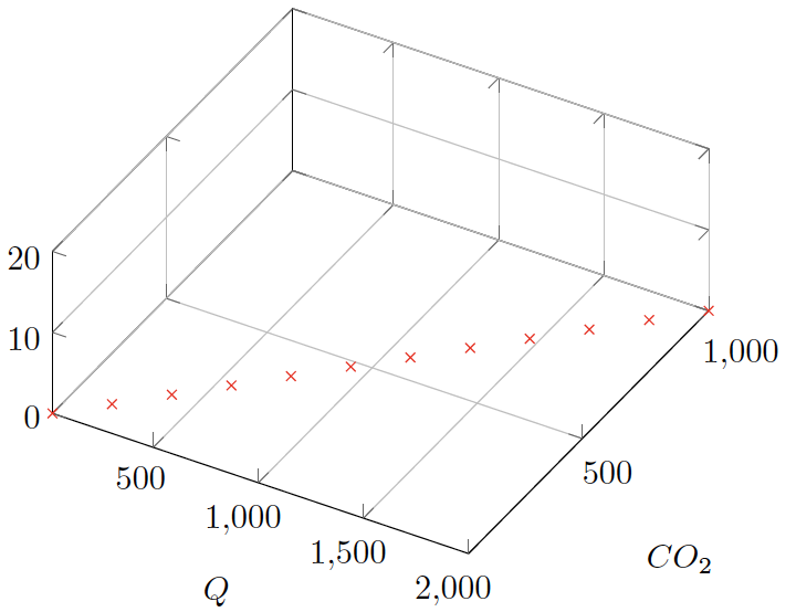
Suppose you want to measure a response surface instead of a curve? For example, photosynthesis, conductance, etc. as a function of light and CO₂. With just 2 independent variables, you could do nested control loops, as illustrated by ../basic/NestedResponse, with a measurement strategy as illustrated by Figure 12‑52. Basically, we are measuring a light curve (lot of points) at a few different CO₂ concentrations.

This would provide four high resolution light curves, and 12 very crude CO₂ response curves. If you want to balance it out, you could work backwards: how much time do you want to spend maximum (say 2 hours), divide it by the average time to equilibrate at each point (say 5 minutes) to get the 24 total points, take a square root (≈ 5), leaving you with 5 light values and 5 CO₂ values. Not very satisfying.

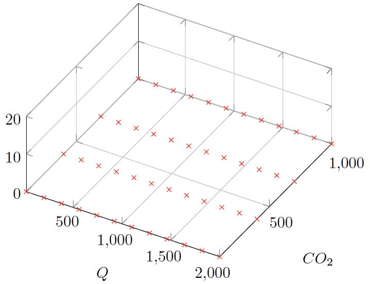
Well, why not use 12 light and 12 CO₂ points, and just one loop, setting both each time (Figure 12‑53)? That way, we could be done in 12 × 5 = 60 minutes.

Plotting out that strategy (Figure 12‑53) makes it clear why it is not helpful: every point we get is on a unique light or CO₂ curve, leaving us with little or no knowledge of what that response surface actually looks like.

But, suppose we use those 12 pairs of points, and randomize the order so that we have a very low correlation between them (Figure 12‑54).

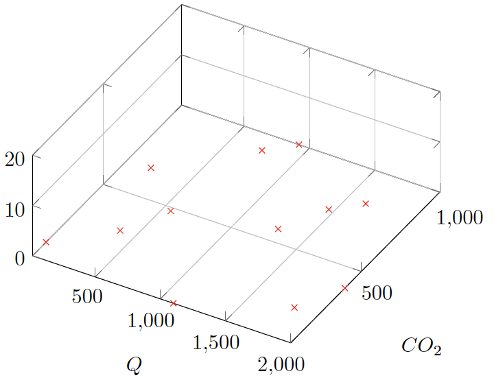
Now we are sampling across the light CO₂ space, and have a chance of getting a reasonable estimate of what the surface above it might be like.

This approach is easy to do with a BP. Let’s start building a program to try this out (Figure 12‑55). We add the list list_utility.py module (an EXEC step), then make two lists of 12 evenly spaced setpoints: q (for light) from 50 to 1500, and c (for CO₂) from 50 to 1000). Another EXEC passes setpoint lists to makeOrtho() to shuffle them, getting back a list of lists, which we put into the original variables. We use SHOW to look at the values.

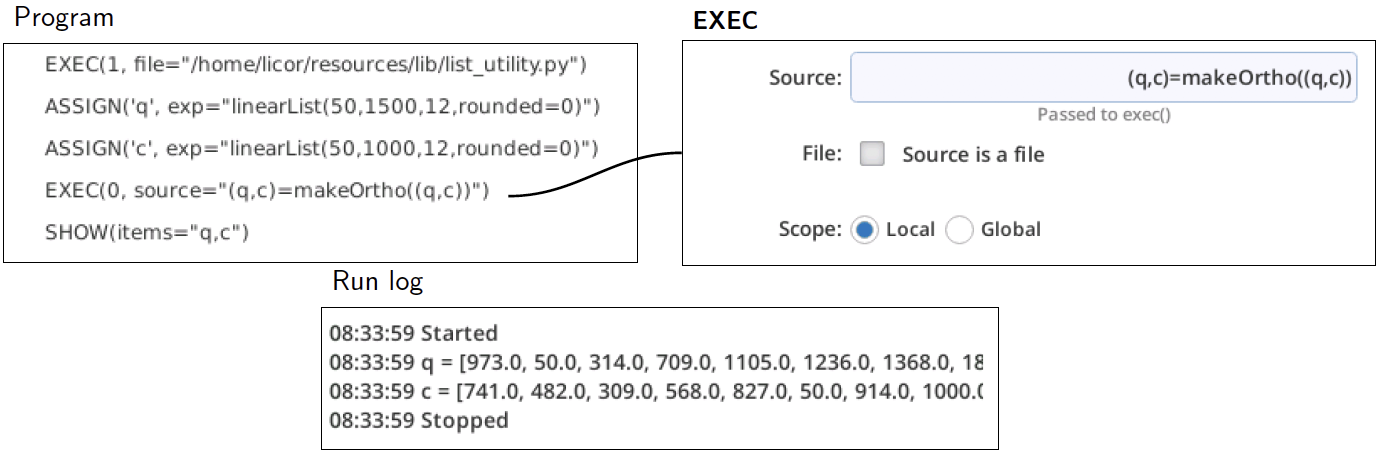
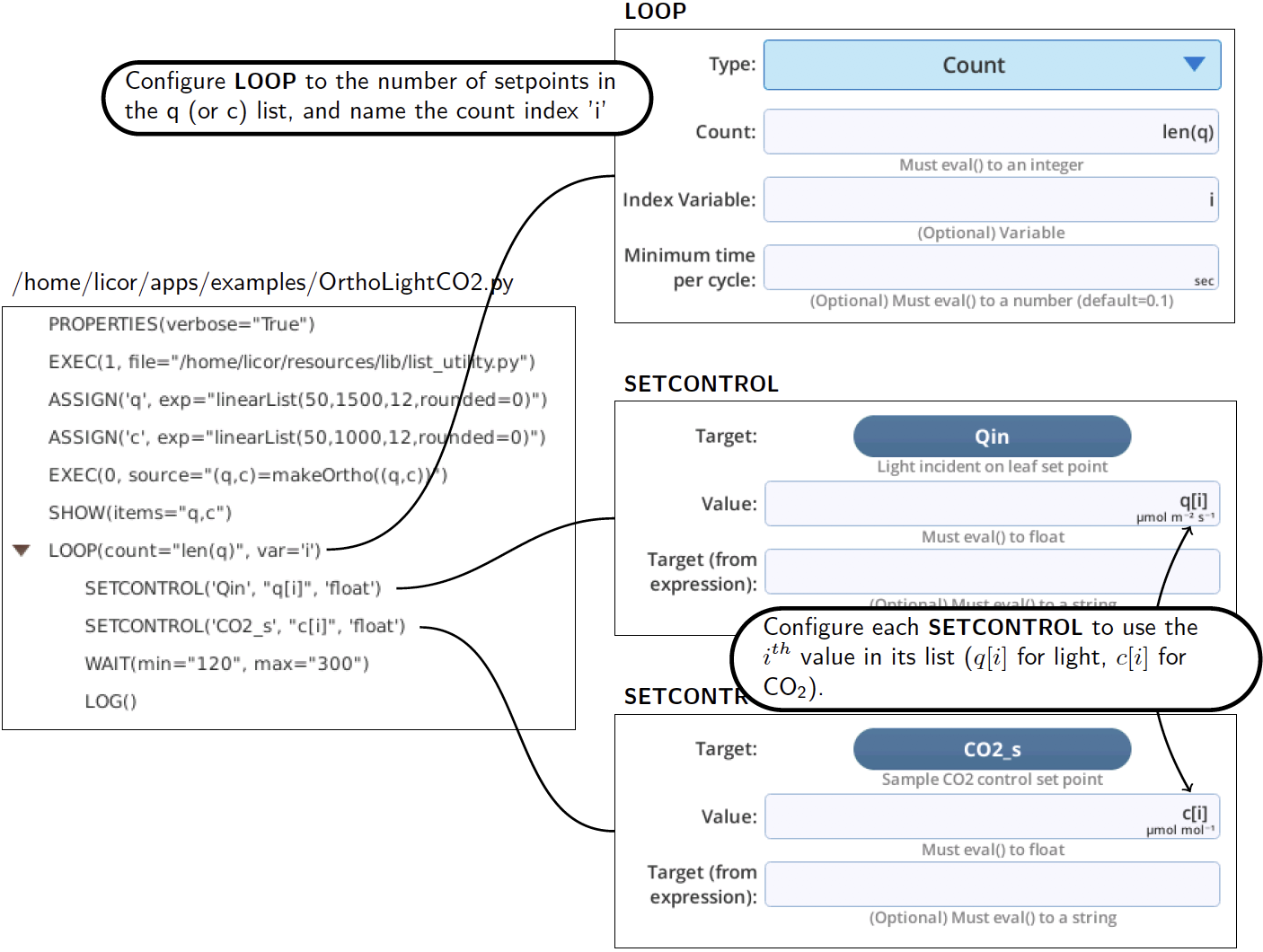
Now all we need is to add a LOOP with SETCONTROLs, WAIT, and LOG, and we have the program /home/licor/apps/examples/OrthoLightCO2.py (Figure 12‑56).

There are two optional parameters provided by makeOrtho() (see The list_utility module), that are illustrated in the following example. Suppose you want three independent variables: light, CO₂, and temperature. Making big jumps in CO₂ or light is not a problem (other than longer leaf equilibration times), but with temperature, you would prefer to make the changes in a monotonic manner as much as possible just to minimize system equilibration time. How can that be done?

An example is /home/licor/apps/examples/OrthoTempLightCO2.py (Figure 12‑57).

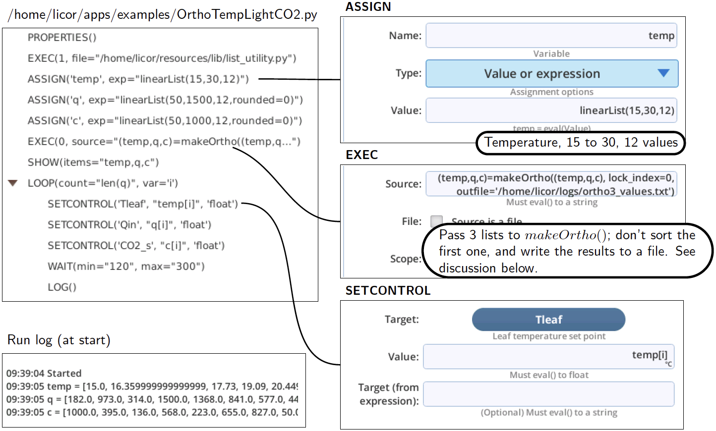
Changes to the previous program are:

(line 3, ASSIGN) - Added a variable (temp) that holds 12 temperature setpoints from 15 to 30.

(line 6, EXEC) - Added temp and some optional parameters to the makeOrtho() call, so it looks like this"

makeOrtho((temp,q,c), lock index=0, outfile='/home/licor/logs/ortho3_values.txt')

lock_index=0 tells makeOrtho() to not randomize the first (0^th) list, which is temp.

outfile='/home/licor/logs/ortho3_values.txt' instructs makeOrtho() to also write its results to a file, so we can view or use these same setpoints later (Listing 12‑2).

Listing 12‑2. Listing of /home/licor/logs/ortho3_values.txt.

(line 7, SHOW) - Added temp to the list.

(line 9, SETCONTROL) - Set leaf temperature to the i^th value of temp.

Variable stability wait times

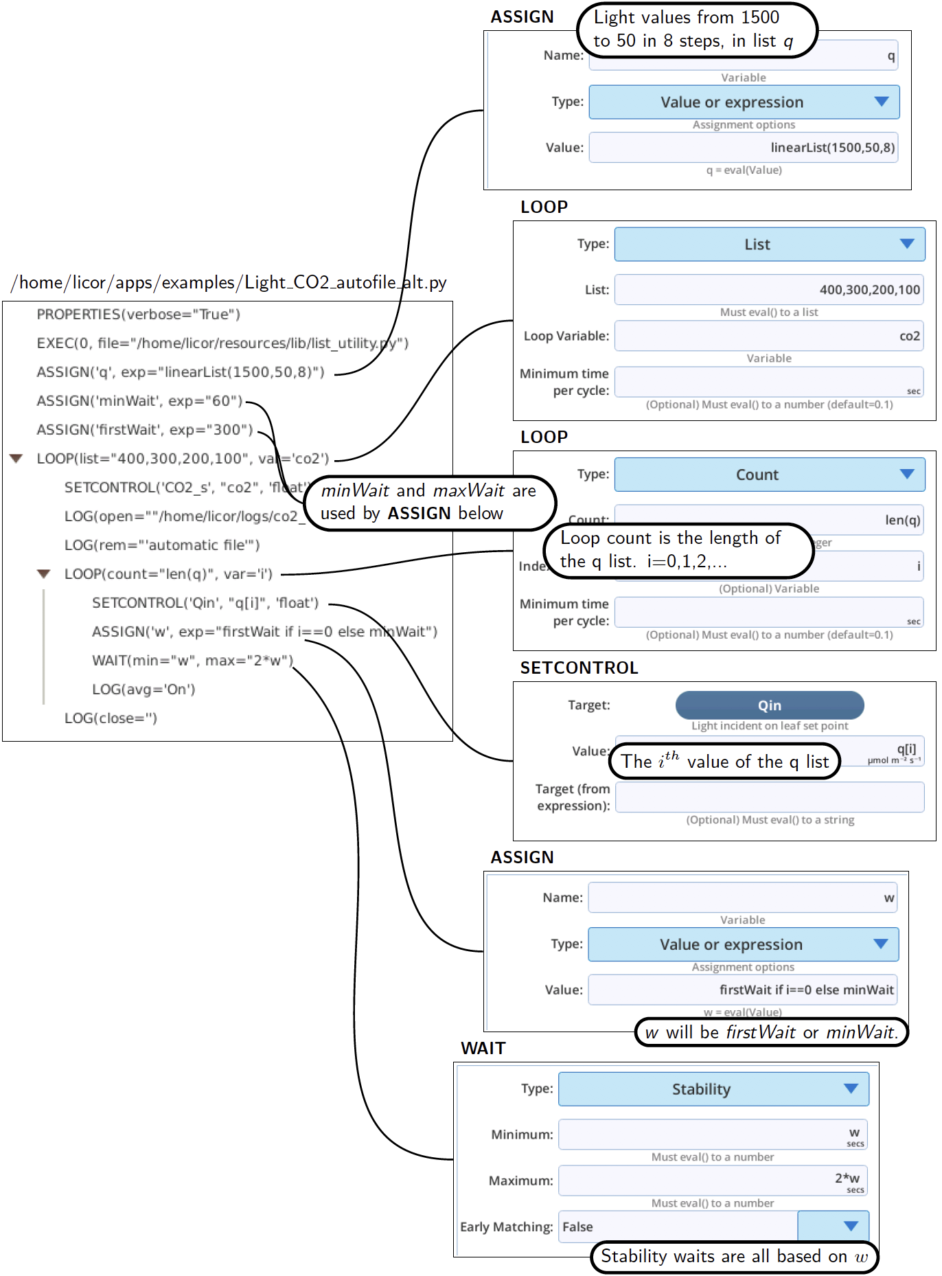
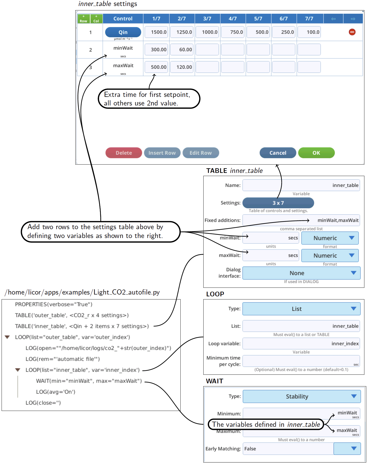
Suppose you wish to do a light curve at a few different CO₂ concentrations by nested loops, with an outer loop that changes CO₂, and inner loop that changes light (the program /home/licor/apps/examples/Light_CO2_autofile.py will do this, putting each light curve in its own log file.) An important consideration with this method is the wait time for the first light value needs to be longer than normal, since the CO₂ will have just changed, and the light will have had a big change from the last value of the previous light curve. A method of accommodating that is shown in (Figure 12‑58).

The equivalent to Figure 12‑58 without using TABLE could be done as illustrated in Figure 12‑59. Here we take advantage of being able to easily generate setpoints (linearList()). minWait is a normal minimum wait time, and firstWait is the time to use on the first pass through the light curve each time. Maximum wait times are always 2 times the minimum.