Why measure CO2 response? An A-Ci curve (assimilation rate plotted against intercellular CO2 concentration) can provide a number of insights into the biochemistry of a leaf or plant, such as:
- CO2 compensation point: The value of Ci where photosynthesis and respiration are in balance.
- Carboxylation efficiency: The initial slope provides an in vivo measure of the carboxylation efficiency. If measuring a C3 leaf, the slope is proportional to the maximum activity of RuBisCO. This is sometimes called the mesophyll conductance.
- Stomatal limitations: Stomatal limitation of photosynthesis can be quantified with CO2 response curves.
- Carboxylation limitations: Within the mesophyll, carboxylation limitations can be separated from electron transport limitations.
CO2 response curve strategies
Below are some things to consider when doing a CO2 response curve.
Light
Light should be held constant and is typically at a non-limiting light level. The LED light source or fluorometer will work just fine for CO2 response curves. Set it to the an intensity that is familiar to the plant and give the leaf some time to acclimate. To determine what light intensity light becomes non-limiting, perform a light response curve and pick the light intensity at Asat.
CO2
In what order should the curve be measured? Consider the parameters that you are most interested in modeling. We recommend starting at ambient and tracking downward toward low concentrations, and then returning to ambient and tracking upwards toward high concentrations. Why? Because at low CO2 concentrations, RuBisCO can be deactivated, while at high concentrations, stomata can close. Avoid spending a lot of time at each extreme. To find ambient CO2, make sure flow is turned on then turn the CO2 and H2O controls off and step away from the console so you aren’t exhaling near the instrument’s air inlet. Look at CO2_r to see approximate ambient CO2. Enter that value as the setpoint.
You also can control CO2_r at "ambient plus the expected delta." The "expected delta" means you add however much to the CO2_r setpoint so that when you close the chamber over a leaf, CO2_s will approximately equal ambient.
Example:
To find what the expected delta is for soybean in a greenhouse you would set the instrument to control CO2_s at the ambient CO2 concentration (let us say it is 400 μmol mol-1), clamp onto a leaf and note the CO2_r concentration when things are stable. If it requires 422 μmol mol-1 to keep the chamber at 400 μmol mol-1, the expected delta us 22 μmol mol-1. Set the instrument to control on CO2_r = 422 μmol mol-1.
The benefit of using this method is that there are no feedback control loops involved for CO2_r and hence the system will reach steady state more quickly. The drawback is that it only works when measuring plants with similar assimilation rates. You probably would not do this if you have large variations in assimilation rates since you want CO2_s to be about the same for each measurement.
Temperature
The response curve should be measured under constant temperature conditions. Operate the coolers at a constant leaf temperature.
Humidity control
For CO2 response curves, use either VPD_leaf set to 1.0-1.5 kPa or RH_air set to 50-85%.
When you set the instrument to control on VPD leaf, if you're not sure of the proper setpoint, clamp onto the leaf with chamber RH between 50% and 70% and check the VPD leaf measurement. A VPD of 1.0-1.5 kPa should keep you in the 50-85% humidity range. Remember that the mixing fan will reduce the leaf boundary layer, but you want the leaf to experience the same humidity in the chamber as it did before it was in the chamber.
Matching
Since the concentrations of CO2 are covering a large range, match before each reading or implement range matching.
This tutorial is a step-by-step guide to manually generating a CO2 response curve. The configuration given below will work well for many plants, but you may need to change the environmental control settings if you are measuring a small leaf or a plant with low photosynthesis rates.
- Set the Environment controls.
-
- Flow: On; Pump Speed: Auto; Flow Setpoint: 500 µmol s-1; and Press. Valve: Manual: 0%. Use a lower flow rate for small leaves or plants with low photosynthesis rates.
- H2O: On; set VDP_leaf to 1.0 kPa
- CO2 injector: On; Soda Lime: Scrub Auto; Set CO2_r near ambient. To find ambient CO2, make sure flow is turned on then turn the CO2 and H2O controls off and step away from the console so you aren’t exhaling near the instrument’s air inlet. Look at CO2_r to see approximate ambient CO2. Enter that value as the setpoint. Controlling on CO2_s will work too but it may take longer.
- Fan: On; Set Fan Speed to 10,000 rpm.
- Temperatures: Check the temperatures to see their current values; Temperature: On; Tleaf: Control at something close to ambient.
- HeadLS or Fluor: For field grown plants, use 1,500 µmol m‑2 s-1; half that much for greenhouse or growth chamber plants. If you don't have a light source, do the experiments in a growth chamber or outdoors. But beware: The experiment is meaningless without steady light.
- Clamp onto the leaf.
- Let the instrument and leaf stabilize for a moment as you go through the remaining steps.
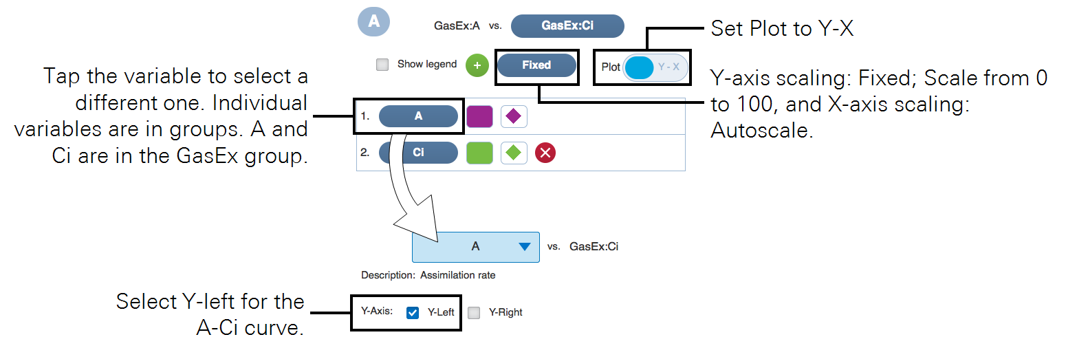
- Set up a graph so you can view the data as they are collected.
- You'll want to plot Assimilation (A) over intercellular CO2 (Ci). Under Measurements, select plot A and then tap Edit Graphs and apply the settings.
- Configure logging options under Log Files and open a log file.
-
- Match Options: Select Always match for this exercise.
- Logging Options: If you are using the fluorometer, set Flr action at log: Nothing. The other settings don't matter for this tutorial.
- Open a Log File: Tap New File. Enter a name, then tap OK. Name the file "Sample CO2 curve," or something similar.
- Wait for measurements to stabilize (not changing much over time), and log the first data point.
- Next, lower the CO2_r setpoint by 100 µmol mol‑1, wait for stability, and then log another point.
- Repeat until done.
- Use these targets for the reference concentration: 300, 200, 100, and 30 (for C3 plants) or 0 (for C4). The last point is designed to be below the compensation point. Notice that the change in CO2 setpoint is accompanied by a brief disruption in the system stability. Try to get 4 or 5 points between your starting value and ending points. Go down to 30 µmol mol‑1 or so for C3 plants, or 0 for C4 plants.
- Finish the curve back at the starting point.
- Set the sample CO2 at the starting setpoint. See how long it takes for photosynthetic rates to return to the original assimilation rate.
- Do some points above ambient, such as 600, 800, 1000, and 1200 µmol mol‑1.
- Review the data.
- Use the graphs to explore the response.
An automatic response curve using the CO2_Response program
Here's how to make an automatic CO2 response curve. It uses an program.
- Set the Environment controls.
-
- Flow, set Flow: On; Pump Speed: Auto; Flow Setpoint: 500 µmol s-1; and Press. Valve: 0.1 kPa
- H2O, set H2O: On; and RH_air: 50 to 75%
- CO2, set CO2 injector: On; Soda Lime: Scrub Auto; Tap CO2_s and enter a setpoint near ambient CO2
- Fan: Set Mixing fan: On; Fan Speed: 10,000 rpm
- Temperatures: On; Tleaf: 27.0 °C or something close to ambient
- HeadLS or Fluor: Use 1,500 µmol m‑2 s-1, or a non-limiting level for your plant.
- Set leaf area and stomatal ratio under Constants > Gas Exchange.
- Configure other gas exchange settings if needed.
- Open a log file.
- Make sure you have the Match Options and Logging Options configured.
- Clamp onto the leaf.
- Under Programs, select CO2_Response.
- Configure the settings or just go with the default settings.
- Tap Start.
- To observe the data as it is collected, set up an A-Ci graph, as described in A manual CO2 response curve. Data are stored in the log file. You can review logged data under Tools > View Log Files. Select the file, then tap Load.