Dynamic Assimilation and curve-fitting: Considerations for fitting DAT CO2 response curves
Authors: LI-COR, Inc.
Correspondence: envsupport@licor.com
Instruments: LI-6800
Keywords: CO2 response curves, curve fitting, dynamic assimilation
Abstract
The Dynamic Assimilation Technique™ (DAT) allows leaf gas exchange measurements to be made when conditions in the leaf chamber are not at steady state. Based on first principles, DAT allows for certain types of measurements to be made that were difficult or impossible to do using steady-state techniques. Further details about the theoretical basis, development, and advantages of this technique are found elsewhere (Saathoff and Welles 2021). In the case of CO2 response curves, a continuously ramping CO2 input can be used to establish varying CO2 concentrations in the leaf chamber instead of several discrete concentrations as is done with steady state measurements. A natural consequence of using DAT with a continuously varying CO2 concentration is that gas exchange data can also be continuously logged. This results in a CO2 response curve with substantially higher data density than a traditional steady-state CO2 response curve. The exact number of points in a DAT CO2 response curve is dependent upon several factors: (1) the logging rate, (2) CO2 ramping rate, and (3) CO2 concentration range that is used, but DAT CO2 response curves generally contain 5-50 times more data than a traditional steady state response curve. This increase in the total amount of data in a CO2 response curve presents some new challenges when fitting Farquhar-von Caemmerer-Berry (FvCB) models of photosynthesis (von Caemmerer 2013) to the curve. Some curve fitting tools are designed to handle data typical of steady state curves and cannot fit the high data density CO2 response curves that are produced from dynamic assimilation. However, other tools, such as R (R Core Team, 2019), do have the capability of fitting DAT CO2 response curves. One popular R package for fitting CO2 response curves is the plantecopys package (Duursma 2015). This package has the advantage of being relatively well documented with a reference manual as well as helpful online guidance (https://remkoduursma.github.io/plantecophys/). Here, we will detail the basic steps for fitting DAT CO2 response curves using the plantecophys package in R.
This guide is not intended to be all inclusive regarding fitting the FvCB model to CO2 response curve data, nor is it intended to cover all fitting options available in the plantecophys package in R. For more details, consult the online guidance referenced above as well as the scientific literature. The package documentation is at: https://cran.r-project.org/web/packages/plantecophys/plantecophys.pdf
1 | Downloading and installing R
R is a freely available program that is widely used by scientists for statistical computing, analysis, and graphing. The base R program has many built in capabilities, and these base capabilities are further expanded by the many user-developed packages that can be installed as an add-on to R. Since R has its own language and is run through a command line interface, new users may want to first familiarize themselves with R and read one of the many introductory tutorials that are available online or through bookstores.
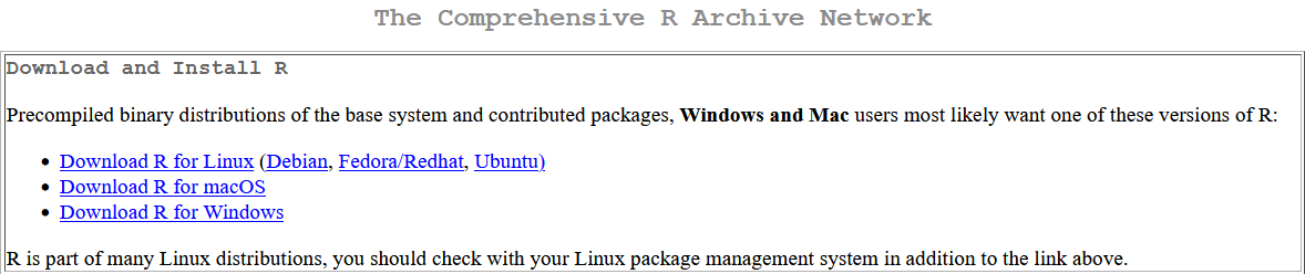
If you do not have R installed on your computer, you can begin by going to the main R website at https://www.r-project.org. R is available for many different types of operating systems, but Windows, Mac, and Linux users should download one of the precompiled binary distributions for ease of installation from one of the CRAN mirrors.
2 | Data formatting and preparation
Data must first be properly formatted before it can be imported into R and used with the 'plantecophys' package. This formatting involves putting the required data for R into properly named columns and then saving the resulting file as a comma separated value (.csv) file. Note that you should use the standard .csv file format and not the UTF-8 .csv format as the latter will not be correctly read by R. A good practice is to put the file into a dedicated directory for importing data into R.
The data file you create for importing into R will contain the following (1) intercellular CO2 (Ci), (2) leaf CO2 assimilation (Photo), (3) leaf temperature (Tleaf), and (4) incident light (PARi). The data file should look like the following.
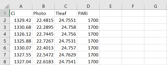
We recommend using the default column names exactly as shown in Figure 2: "Ci", "Photo", "Tleaf" and "PARi". This file should then be saved into your designated R import directory as a .csv file using the Save As option.
If you already have experience using R, note that it is possible to load the text version of a LI-6800 data file into R directly. However, doing so requires developing a custom function that can parse the data file into named vectors that are then accessible by the curve fitting routine.
3 | Downloading the plantecophys package
If you have newly installed R on your computer, or if you have not used the plantecophys R package, you will first need to install the package so it can be used by R. The computer must be connected to the internet to do this. Installing the package requires the following command:
> install.packages("plantecophys")Typing the above command into the R command line interface will tell R to download the package from the CRAN servers. Note that R code, like many others, is case-sensitive.
4 | Loading the package into R
Once the plantecophys package has been downloaded, it needs to be loaded into R by using the following command:
> library(plantecophys)5 | Fitting the CO2 response curve
The process of fitting the CO2 response curves to the FvCB model requires a couple of steps. The first step is to load the CO2 response curve data into R and give the data a name. The second step tells R to fit the data using the plantecophys package. These steps are detailed below.
Step 1: Load your data into R. Here, we show how to load a file called SoyCurve1 into R and name the data Aci1.
> Aci1 <- read.table("c:/Rdata/SoyCurve1.csv", header=TRUE, sep=",")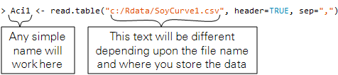
Alternatively, if you have already set the working directory in R and have placed your .csv file in that directory, you can import data using the following command:
> Aci1 <- read.csv("SoyCurve1.csv")Step 2: Fit the named data set using the fitaci function. The command to do so is:
> f <- fitaci(Aci1)
Step 3: Plot the fit results to verify they look appropriate.
> plot(f)
Step 4: If the fit looks appropriate, you can generate a summary table, or you can simply look up the output from the fitaci function.
> summary(f)The summary command will include a table like this:
| Estimated parameters: | ||
| Estimate | Std. Error | |
| Vcmax | ||
| Jmax | ||
| Rd | ||
| Note: Vcmax, Jmax are at 25C, Rd is at measurement T. | ||
| Curve was fit using method: default | ||
The above table contains the estimates for Vc,max, Jmax, and Rd. TPU limitation was not fit. If multiple curves are being fit, it is possible to fit them using the fitaci function with a summary generated for all of the curve fits.
6 | DAT curve fitting considerations
CO2 response curves can provide detailed physiological insight into limitations on photosynthesis (Long and Bernacchi 2003). In general, for any CO2 response curve, it is very important to inspect the fit results for CO2 response curves to make sure they are believable and reasonable. For high data-density CO2 response curves, inspecting the results becomes even more important to ensure that the transition point between Rubisco and RuBP-regeneration limited regions of the response curve is appropriately specified and that the model fit looks appropriate. If the fit does not appear appropriate, it may be necessary to adjust the data used for fitting, especially in cases where TPU limitation may be present.
In the example below, data is shown from a CO2 response curve conducted on soybean. The curve was conducted with a 1605 – 5 µmol mol-1 CO2 ramp at a ramping rate of 200 µmol mol-1 min-1. Actinic light was set to 1700 µmol m-2 s-1, chamber air temperature was controlled at 25 °C, and relative humidity was set to 60%.
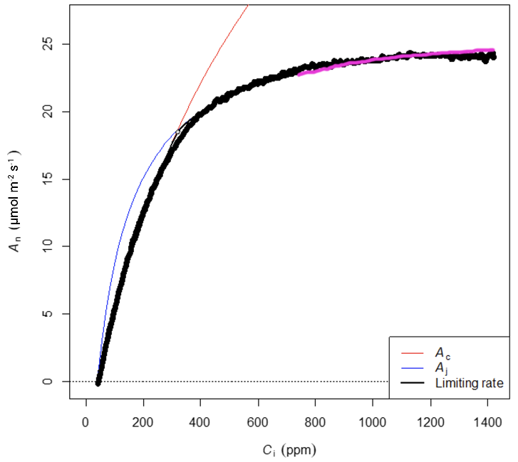
The first attempt to fit the data used the entire data set and yielded the following results (Figure 3).
| Parameter | Value | Error |
|---|---|---|
| Vc,max (µmol m-2 s-1) | 69.0 | 0.25 |
| Jmax (µmol m-2 s-1) | 113.6 | 0.22 |
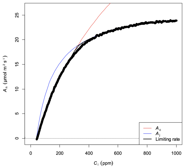
The parameter estimates looked reasonable, although visual inspection (Figure 3) showed that the curve fit in the RuBP-limited region of the curve could be improved a little. This was evident because the fit was underestimating the response at Ci values between 600-800 µmol mol-1 and overestimating the response at Ci values greater than 1200 µmol mol-1 (Figure 3; magenta highlighted line). Furthermore, the pattern was consistent with TPU limitation (Long and Bernacchi 2003, Sharkey 2019). The apparent TPU limitation above Ci values of about 1000 µmol mol-1 was distorting the overall fit. By limiting the data to Ci values below 1000 µmol mol-1, a better fit was obtained (Figure 4).
| Parameter | Value | Error |
|---|---|---|
| Vc,max (µmol m-2 s-1) | 69.2 | 0.24 |
| Jmax (µmol m-2 s-1) | 114.6 | 0.22 |
The parameter estimates (Table 2) did not change very much, but this would be expected because the apparent misfit was small to begin with. Additionally, the TPU limited region appeared at relatively high Ci above 1000 µmol mol-1; if the TPU limited region were larger – thus reducing the region where J is limiting – then the initial fit would have had a larger error and more data would need to be excluded in order to obtain a good fit. In turn, the parameter estimates (particularly Jmax) would have likely shown more change after fitting the reduced data set.
Finally, it is possible to directly fit TPU limitation using the following command:
> f <- fitaci(Aci1, fitTPU=TRUE)A word (or several) of caution: using the TPU-fitting option for a DAT curve can sometimes dramatically lengthen the time required for the fit to complete due to the much higher data density inherent in DAT response curves. Also, note that fitting TPU forces the algorithm to use a different fitting method that will result in parameter estimates that are likely to be slightly different from estimates obtained using nonlinear least squares. Additionally, not all parameters will have an error estimate associated with them when the TPU fitting option is used. This is problematic because parameter error is useful in determining how precise the parameter estimate is.
The fit results using the fitTPU=TRUE option follow below (Figure 5).
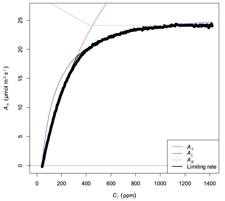
The results show parameter values (Table 3) that agree with the other estimates obtained previously. However, unless VTPU is a parameter of interest, it is advisable to simply fit data up to the point where TPU limitation becomes apparent because of the time penalty that can be incurred when using the TPU fitting option with high data density CO2 response curves.
| Parameter | Value | Error |
|---|---|---|
| Vc,max (µmol m-2 s-1) | 69.0 | 0.28 |
| Jmax (µmol m-2 s-1) | 114.0 | NA |
| VTPU (µmol m-2 s-1) | 7.9 | NA |
7 | References
| 1 | Duursma, R. A. (2015). Plantecophys - An R package for analysing and modelling leaf gas exchange data. PLoS ONE, 10(11), e0143346. doi:10.1371/journal.pone.0143346 |
| 2 | Long, S. P., & Bernacchi, C. J. (2003). Gas exchange measurements, what can they tell us about the underlying limitations to photosynthesis? Procedures and sources of error. Journal of Experimental Botany, 54(392), 2393-2401. doi:10.1093/jxb/erg262 |
| 3 | R Core Team. (2019). R: A language and environment for statistical computing. Retrieved from https://www.R-project.org/ |
| 4 | Saathoff, A. J., & Welles, J. (2021). Gas exchange measurements in the unsteady state. Plant, Cell & Environment, 44(11), 3509-3523. doi:10.1111/pce.14178 |
| 5 | Sharkey, T. D. (2019). Is triose phosphate utilization important for understanding photosynthesis? Journal of Experimental Botany, 70(20), 5521-5525. doi:10.1093/jxb/erz393 |
| 6 | Von Caemmerer, S. (2013). Steady-state models of photosynthesis. Plant, Cell & Environment, 36(9), 1617-1630. doi:10.1111/pce.12098 |