A quick introduction
Version 1.5 supports a more general form of the flux equations for assimilation and transpiration, relaxing the requirement that the system be in steady state (rate of change of CO2 and H2O at or near zero). The details about the equations and how they have been implemented are contained at the end of this section (Dynamic details); what follows here is a practical introduction and guide.
Benefits
The advantage of using the dynamic equations is that it removes the requirement that the chamber conditions be in steady state. Figure 9‑33 shows the results of doing step changes in CO2 between 400 and 500 µmol mol-1 every 1 minute with a closed, empty chamber. Asty (assimilation computed with the steady state equation) spiked to ±40 µmol m-2 s-1, returning to the true flux 0 in about 45 seconds. Adyn (assimilation computed with the dynamic equation) spiked to less than 1.5 µmol m-2 s-1, returning to the true flux in about 15 seconds.
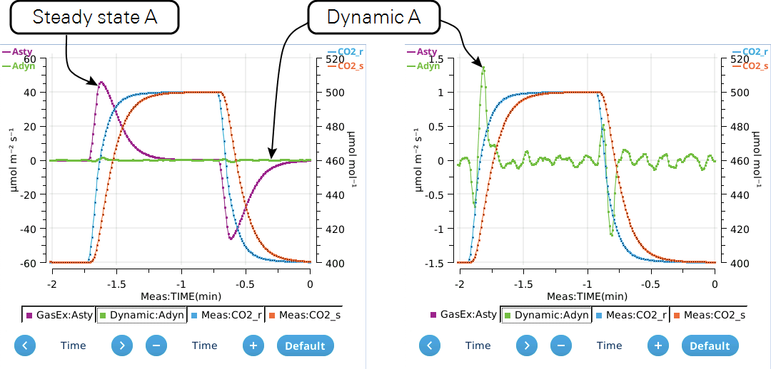
Figure 9‑34 is also an empty chamber experiment, this time with CO2 being ramped up and down at one minute intervals between 400 and 500 µmol mol-1. Asty is high by 10 µmol m-2 s-1 when CO2 is ramping up, and low by the same amount when ramping down. Meanwhile, Adyn generally stays within ±0.1 µmol m-2 s-1.
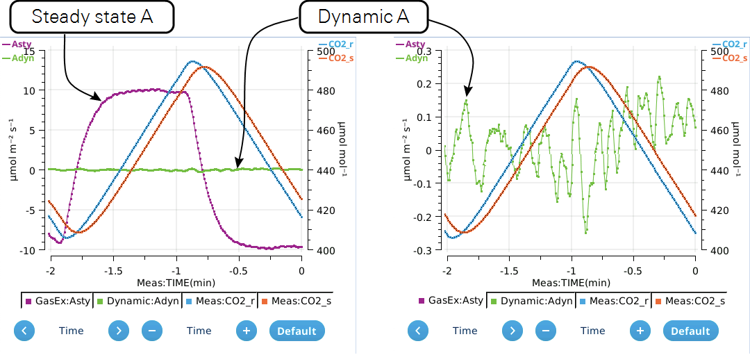
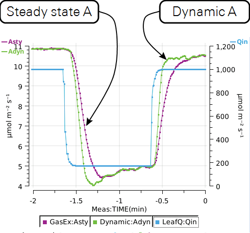
Figure 9‑35 compares Asty and Adyn while measuring a leaf exposed to a brief drop in light intensity. Here, CO2 reference is being controlled, and changes in chamber CO2 concentration come from changes in light intensity. Reduced light reduces assimilation which increases chamber CO2, causing Asty to be higher than Adyn (just like when CO2 is ramping up in Figure 9‑34; the reverse happens when light increases.
Consideration 1: Range matching
In a steady state measurement, you want the analyzers to be matched at the concentration at which you are operating. In a series of non-steady state measurements, the concentration is continually changing, so the analyzers have to be matched at not just one concentration but over a range of concentrations. This is easily achieved in the LI-6800 by implementing its range matching feature.
Consideration 2: Dynamic tuning
There are extra parameters involved in the dynamic computation that need to be known before-hand. These parameters depend on chamber and flow rates (flow to chamber and flow to reference IRGA). When these parameters are tuned correctly, the dynamic equations will give the proper result no matter if the concentration is linearly increasing or decreasing, regardless (within reason) of how fast it is changing. For a detailed look at these parameters, see Three tuning parameters.
For each chamber that supports dynamic equations, the system has a built-in look-up table for these parameters that are intended to serve as a reasonable first guess. So with no further action on your part, you should get reasonable dynamic values. This built-in look-up table is referred to as the Sys table.
It is very easy to check the validity of the dynamic system's look-up table to your instrument: built-in tests are provided that use a closed, empty chamber (flux is zero) and ramp the concentration up and down several times. Computed dynamic fluxes should be the same (0, if properly range matched) regardless of ramp direction. If not, the best fit values are computed and go into a separate look-up table know as the User table. This "tuning" process takes a couple of minutes for one flow rate, and is recommended prior to performing a rapid A-Ci curve, where you are depending on the accuracy of the dynamic flux computations.
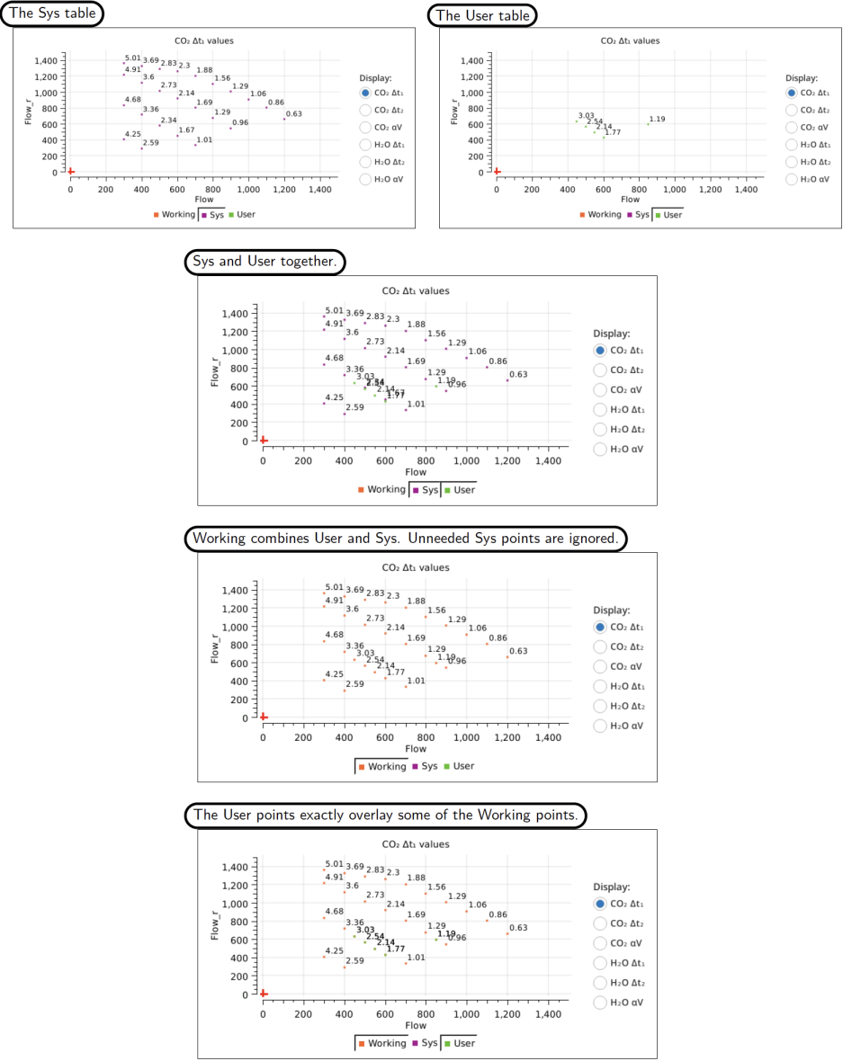
The Sys and User tables combine to form the Working table, which is simply the Sys table plus the User table, with the User table entries taking priority over Sys table entries. See Figure 9‑47 and Figure 9‑48.
Consideration 3: Noise
In steady conditions, the dynamic formulation is potentially noisier than the steady state one, because of the rate of change term (see Equation derivation). When conditions are steady, this slope is small, but bounces around contributing noise.
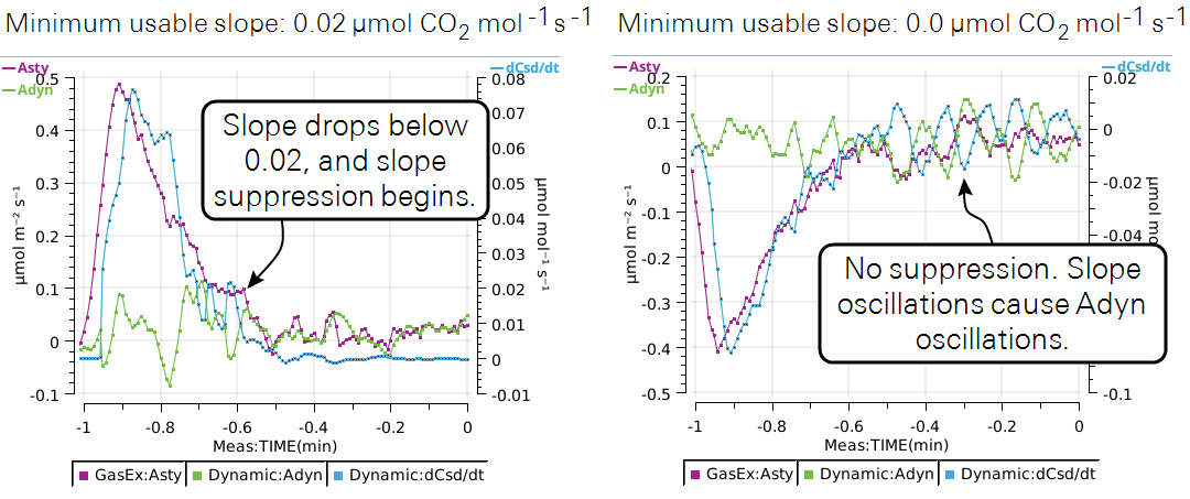
To address this, the LI-6800 uses a "minimum usable slope" value, which should be set to a level just above the slope values you would expect in a closed, empty chamber. (The default values are 0.02 µmol CO2 mol-1 s-1 and 0.005 mmol H2O mol-1 s-1.) While the absolute value of the slope remains below this value, the slope value actually used in the dynamic computations is suppressed by increasing amounts as time progresses. The suppression is done by dividing the slope by (1 + t / 2), where t is the number of seconds the slope has been consistently below the threshold. After 10 seconds, for example, the slope used in the computations is 1/6 of its real value; after 20 seconds, it is 1/11 of its real value. This increasingly damps the noise and brings the dynamic performance in line with the steady state performance. The first time the actual slope exceeds the minimum usable value, however, t resets to 0, so there is no hold-over effect.
"Minimum usable slope" is illustrated in the empty chamber experiments shown in Figure 9‑36. Each shows 1-minute strip charts following a 1 ppm change in reference CO2. The blue lines are sample CO2 slope, the red lines are Asty (steady state assimilation), and the green lines are Adyn (dynamic assimilation). With slope suppression (left) the noise of Adyn and Asty become comparable following the perturbation. Without it (right), they are not.
Using DAT
Enabling and disabling
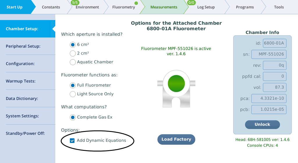
If dynamic equations are available for a chamber/configuration, an Options group will appear on the Chamber Setup page (Figure 9‑37). Check the box to add the dynamic equations and enable related interface support pages.
Steady state or dynamic?
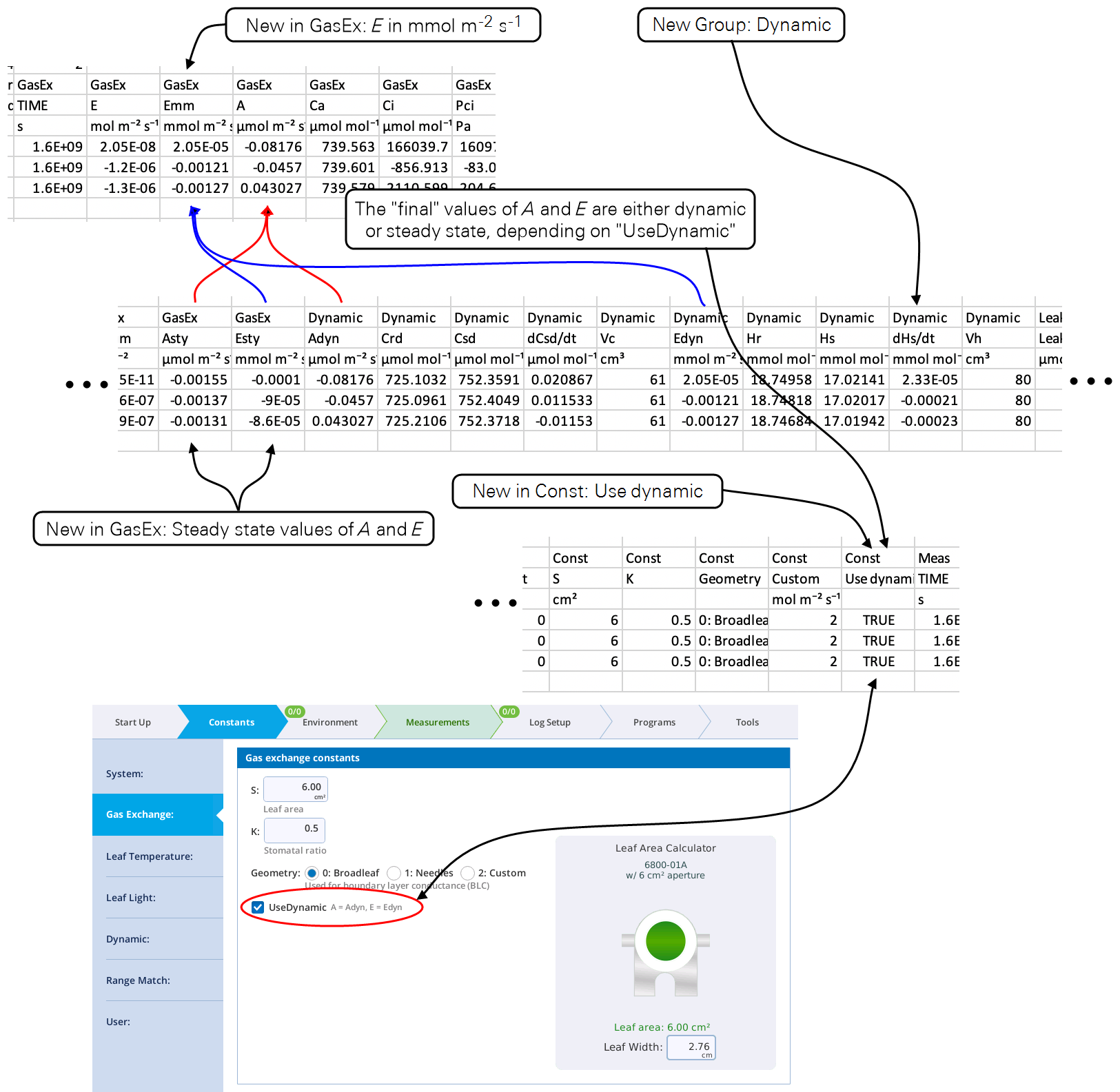
When dynamic equations are included, both steady state and dynamic fluxes are provided; you can decide (before or after logging) which method you wish to use. The dynamic fluxes Adyn and Edyn and related inputs are provided in a new group, named Dynamic. The GasEx group has added two new entries, Asty and Esty, which are the steady state values. The traditional fluxes, A and E in GasEx now come from either Asty and Esty, or Adyn and Edyn.
Figure 9‑38 illustrates how this works; when dynamic equations are added, there is a checkbox on the GasEx constants page that determines whether the final fluxes A and E are steady state or dynamic. That checkbox corresponds to the "Use dynamic" entry in the Gas Exchange constants group (Const), which is also present in the Excel file, allowing you to make the steady-state vs dynamic determination after-the-fact.
Get a quick overview
Constants > Dynamic > Current Status (Figure 9‑39) lets you view and compare the real time steady state values (Asty and Esty) with the dynamic (Adyn and Edyn), and the major inputs that the dynamic values use, including the fit coefficients from the Working table.
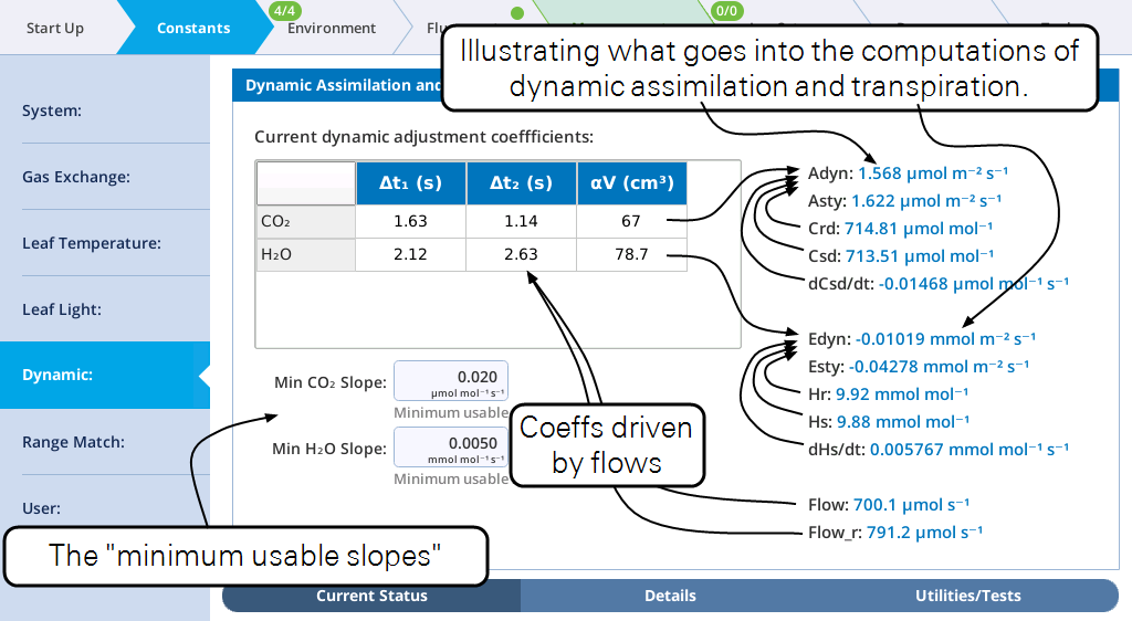
The table in the upper left shows the current values of the coefficients. They will change as flow rate changes (and if you change chambers). These values come from look-up tables, which you can view (Visualizing the look-up tables) and modify (described in How good are the coefficients?).
How good are the coefficients?
Constants > Dynamic > Utilities/Test (Figure 9‑40) provides methods for testing and improving the dynamic coefficients. It does this by measuring a known flux rate (zero, because the chamber is empty) while cycling CO2 (or H2O) up and down for a couple of minutes, then computing dynamic flux, first with the existing coefficients, then doing a best fit on the data to improve the coefficients. See The dynamic tests for more details.
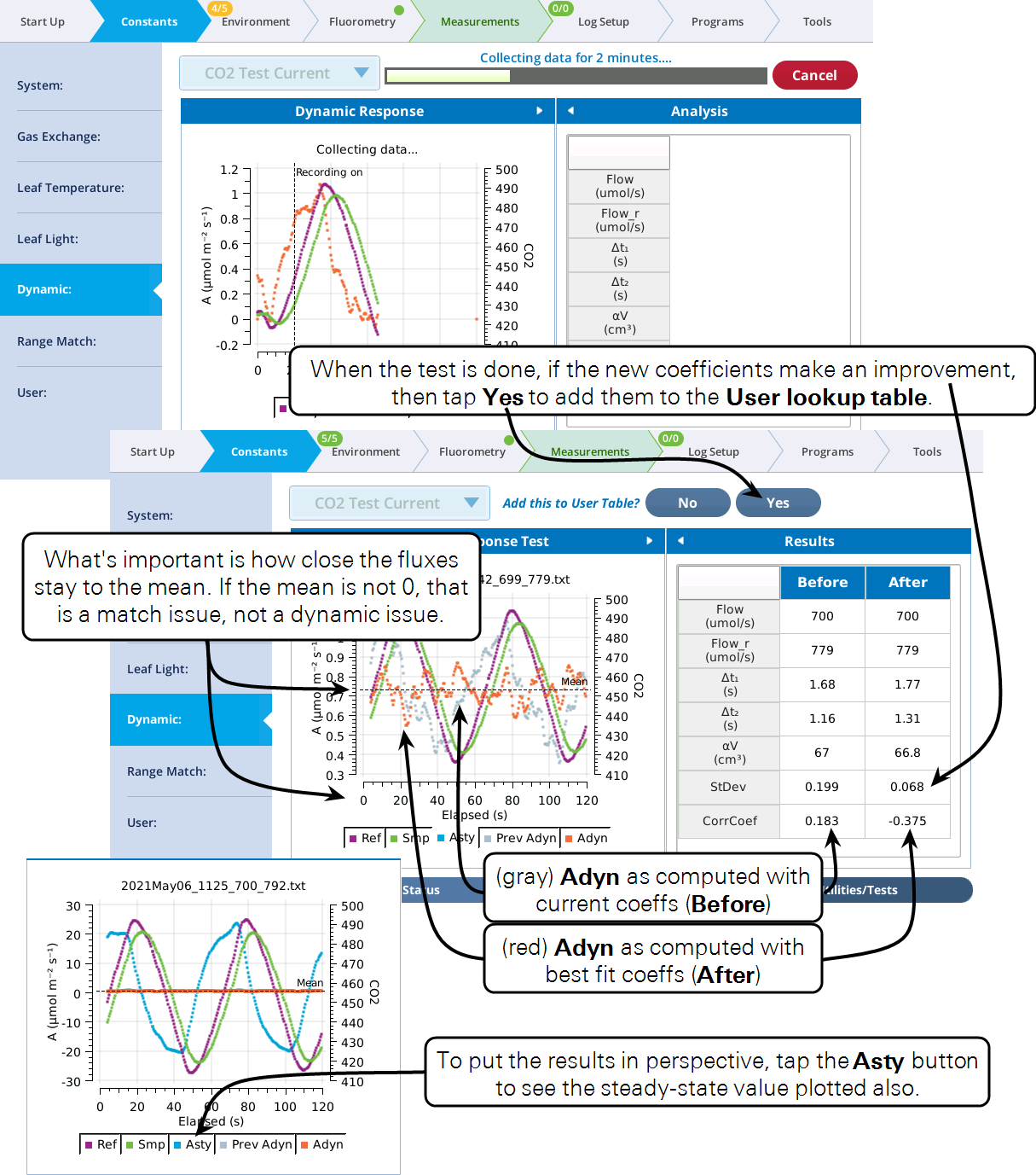
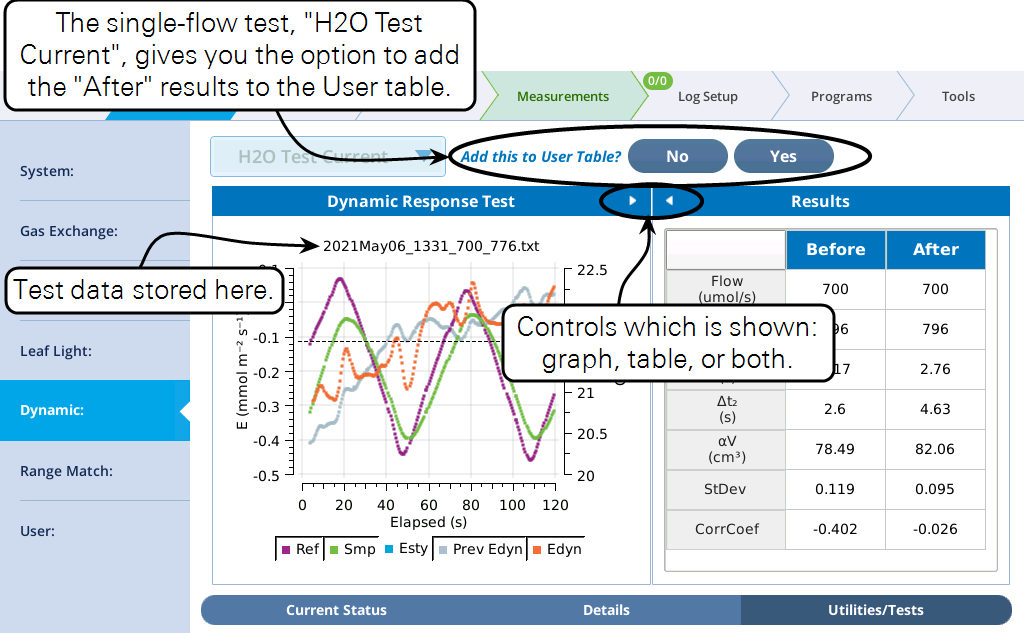
While the test runs (top of Figure 9‑41), dynamic flux is plotted along with sample and reference concentrations. Ideally, there would be no correlation between the concentrations and the flux. When the test is completed (bottom of Figure 9‑41), the standard deviation of the dynamic flux and the correlation coefficient between flux and sample concentration is computed and displayed in the table (the Before column). Finally, best fit (minimizing the sum of squares between dynamic flux about its mean) values for Δt1, Δt2, and αV are computed, along with the stats of those results, and displayed in the table's After column.
If the "After" stats are better (lower standard deviation) than the "Before" stats, then you can add this result to the User table by tapping the Yes button. Otherwise, tap No.
Making a rapid A-Ci curve
Below is a suggested protocol for making rapid A-Ci curves with the dynamic method.
- Let the instrument warm up thoroughly and adapt to the ambient temperature (e.g., 2 hours).
- Check CO2 and H2O range matching.
- Determine the flow rate you will be using for the A-Ci curve.
- Do dynamic tuning for CO2 by running "CO2 Test Current".
- (optional) Do H2O tuning by running "H2O Test Current".
- Open a log file.
- Do the experiment using one of the three DAT background programs described below. Note that the logging triggered from these programs uses the following overrides:
- Matching is suppressed for both CO2 and H2O.
- Fluorometer events are turned off.
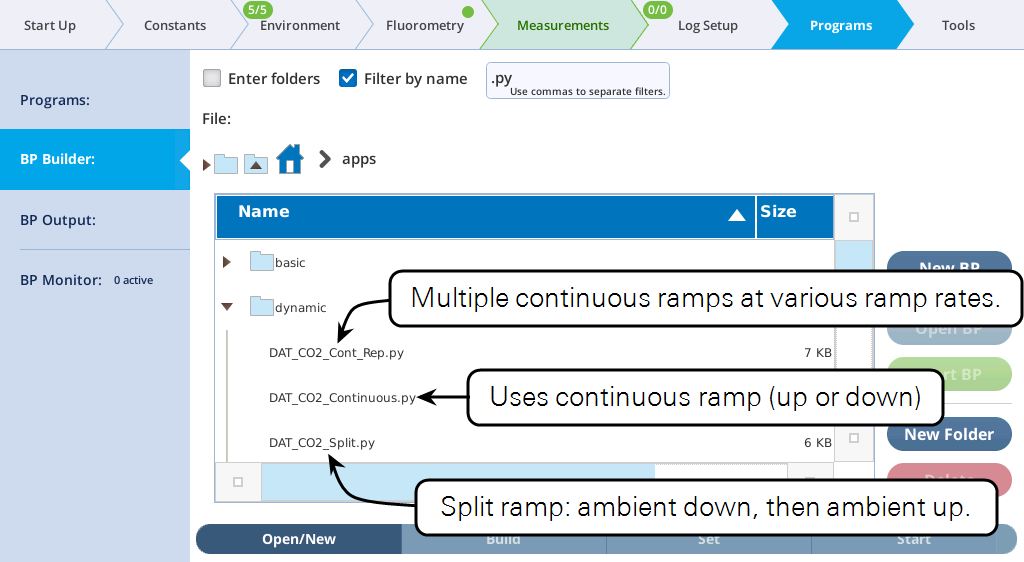
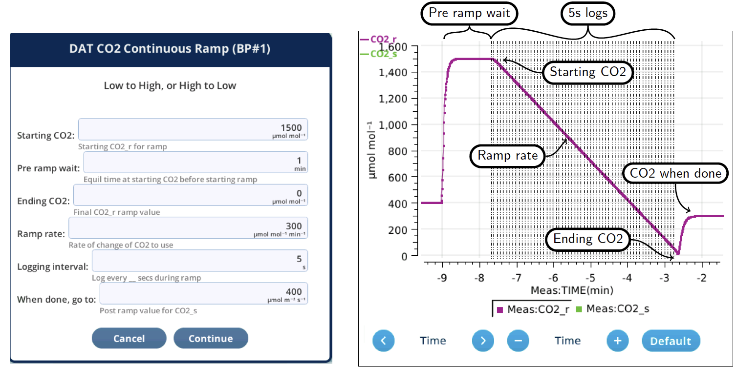
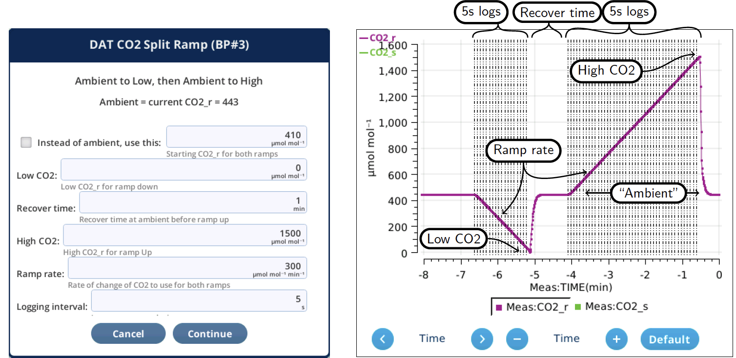
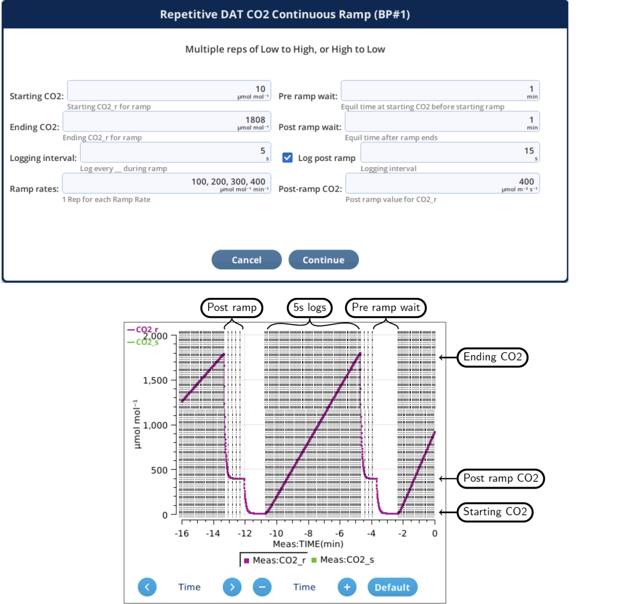
Three background programs designed for measuring rapid A-Ci are found in /home/licor/apps/basic: To measure an A-Ci curve in one continuous ramp (up or down), use DAT\_CO2\_Continuous (Figure 9‑43). To do this repetitively, use DAT\_CO2\_Cont\_Rep (Figure 9‑45). To start at ambient and go down, then recover and ambient then ramp up use DAT\_CO2\_Split (Figure 9‑44).
Note that all three of these programs automatically set Log Options for additional averaging at a time that matches your logging interval. This gives you the benefit of having your logged data reflect all the measurements, but without having to log at an impossible frequency.
Recomputing DAT in Excel files
There are three dynamic tuning parameters involved in the computation of a dynamic flux: Δt1 and Δt2 are time offsets for the reference concentration and the slope computation, and αV is the effective volume (see Three tuning parameters). Only the αV parameter is saved in Excel files, as part of the Dynamic group (αVc for CO2 and αVh for H2O). The other two parameters (Δt1 and Δt2) have already been used to come up with the reference and sample concentrations, and the rate of change terms, so it is too late to change those in the Excel file.
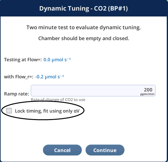
This has the following implication for rapid A-Ci curves: if you failed to do proper dynamic tuning before the A-Ci curve was generated, you could still do it after the fact and recompute, but make sure that:
- You use the same flow rate.
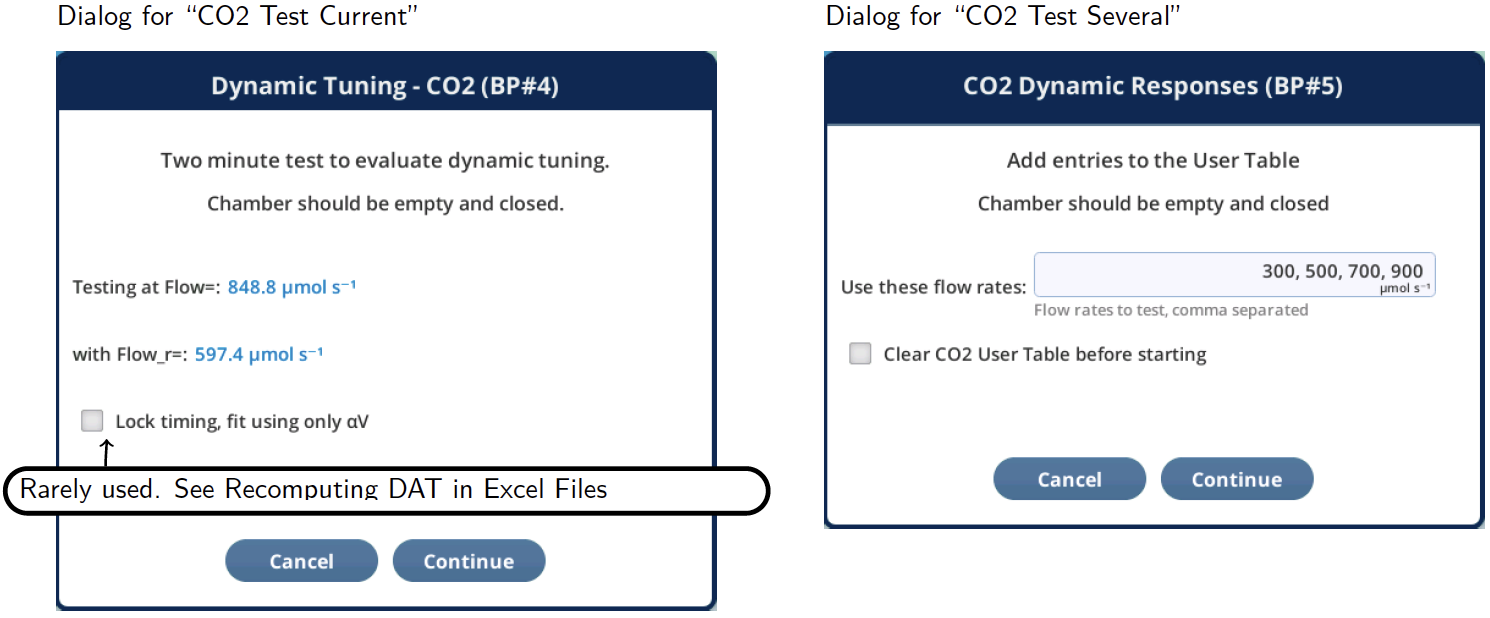
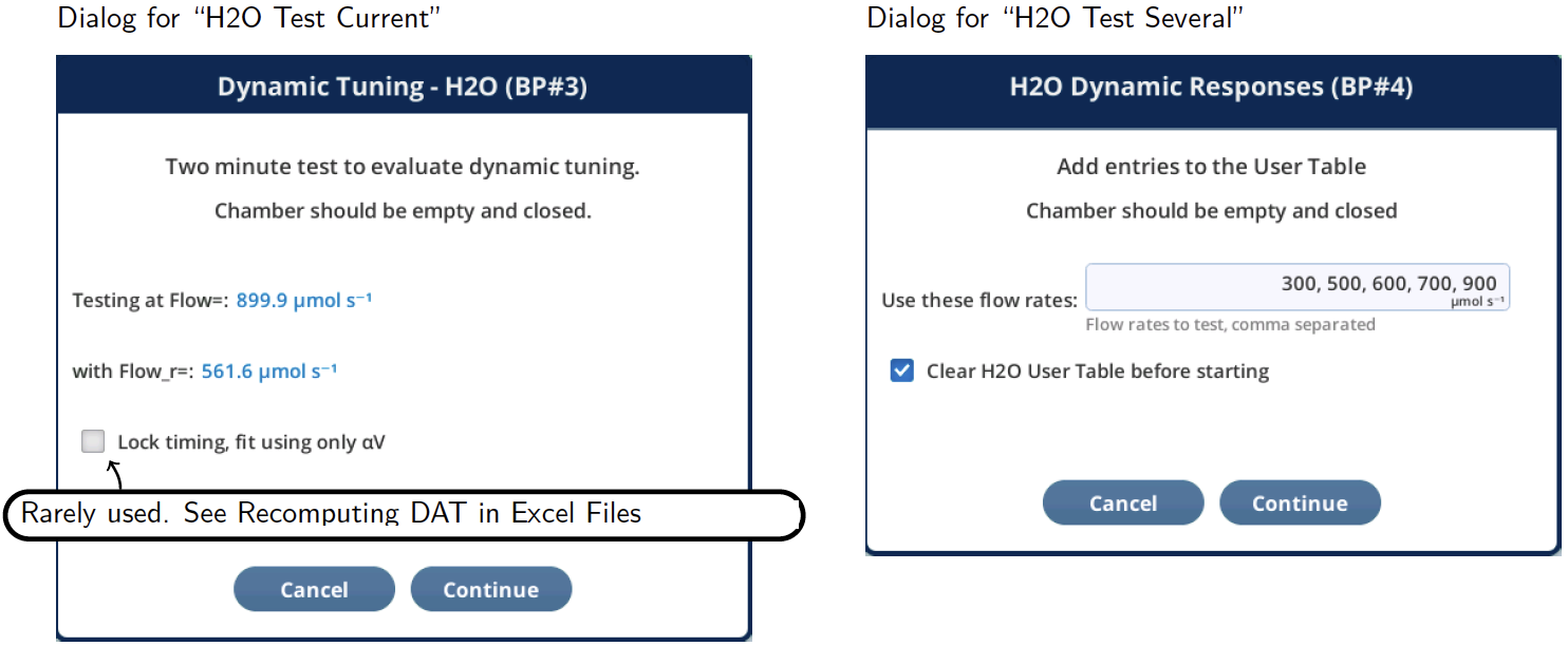
- Run "CO2 Test Current", and check the "Lock timing" box (Figure 9‑46). This forces all of the tuning correction into the αV term.
- Use the "After" αV value in the Excel file for the Dynamic:Vc value.
Visualizing the look-up tables
Constants > Dynamic > Details (Figure 9‑47) allows you to view the look-up tables that are used to determine dynamic coefficients for various flow rates. Tables can be viewed as a table or as a map. In fact, there are three tables for each of CO2 and H2O, named Sys, User, and Working.
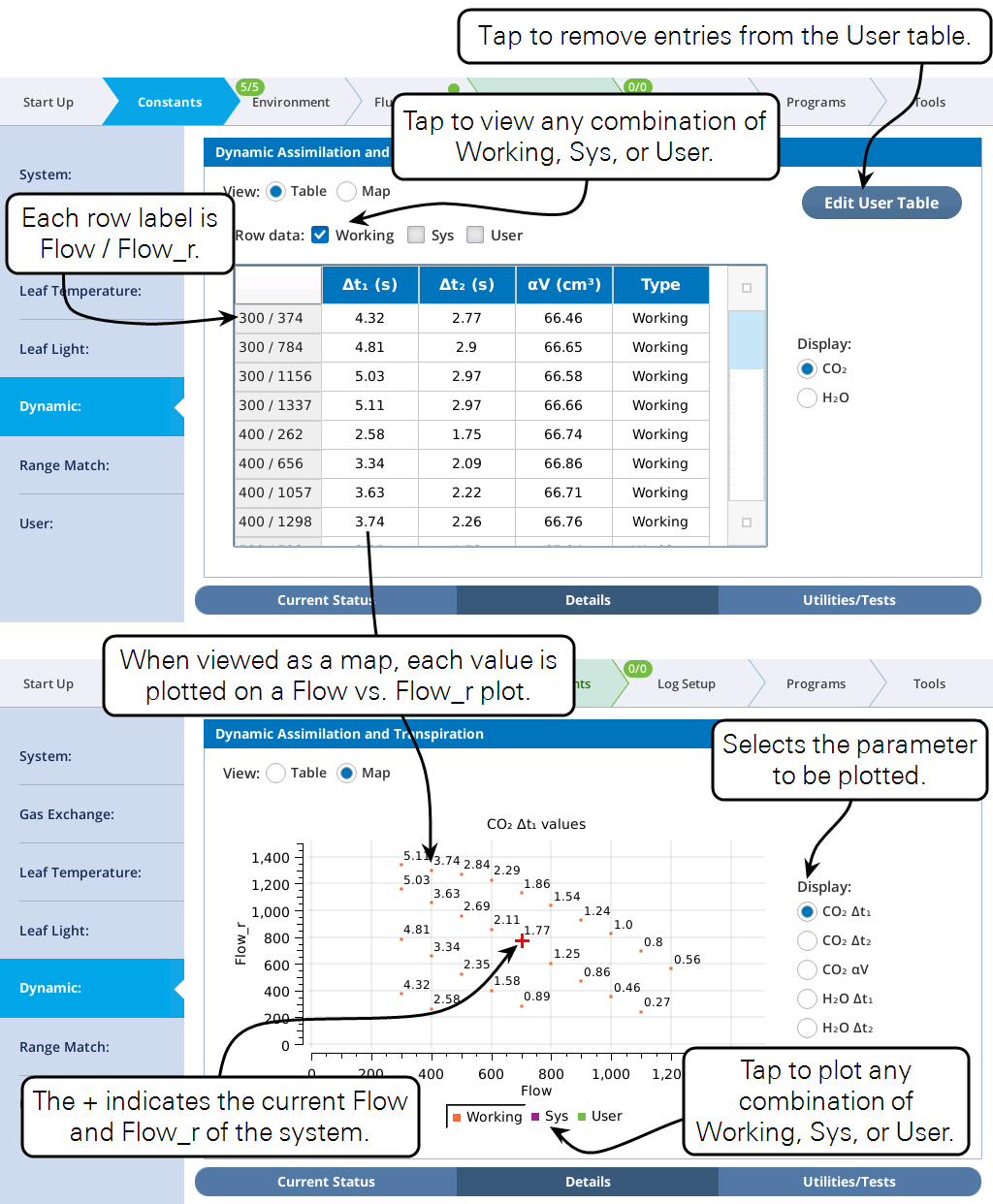
The map view (Figure 9‑48) illustrates how the Sys and User tables are combined to make the Working table
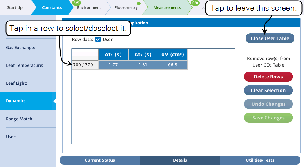
User tables can be edited by tapping the Edit User Table button (Figure 9‑49). Tap in the row(s) of entries you wish to select. Delete selected rows by tapping the Delete Rows button. Save Changes makes the changes permanent. Tap Close User Table to leave the editor.
Entries that have been removed can be restored to the User table by using the "CO2 Reload" or "H2O Reload" utility in the Utilities/Tests screen (Reloading a test).
Dynamic configuration elements
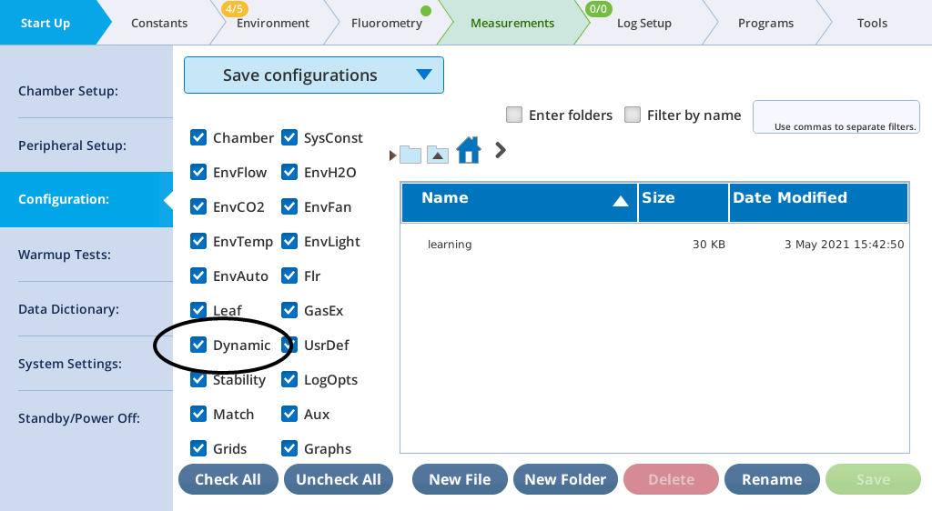
When Dynamic equations are enabled, there is a Dynamic topic available when storing and loading configuration files (Figure 9‑50). This includes the CO2 and H2O minimum usable slopes and user table entries. Note the table entries are specific for the attached chamber. If you save a configuration file for one chamber type, and reload that file when a different model chamber is attached, the table entries are ignored.
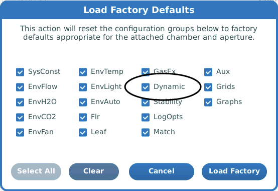
There is also a Dynamic entry in the Load Factory Defaults dialog available from Start Up > Chamber Setup screen (Figure 9‑51). The effect of loading Dynamic factory defaults is to reset the minimum usable slopes to default values (0.02 for CO2 and 0.005 for H2O), and clearing any user table entries for CO2 and H2O.
The dynamic tests
CO2 test description
Testing the CO2 dynamics is performed by using a closed, empty chamber and putting the CO2 reference control into a series of ramps up and down, each ramp lasting 30 seconds. The low ramp value is 400 ppm, the upper ramp value is 400 + r / 2, where r is the ramp rate in ppm / minute. 20 seconds after the ramping is started, data is collected for 2 minutes.
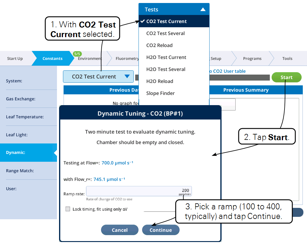
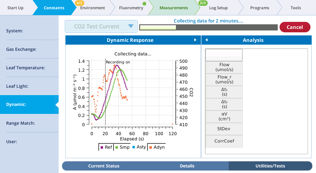
Two CO2 tests are provided (Figure 9‑52): "CO2 Test Current" performs the test at the current flow rate, and at the end gives you the choice of adding the result to the User table. "CO2 Test Several" runs the test on a range of flow rates, and automatically put the results into the User table.
While data is being collected (Figure 9‑53), concentrations and fluxes are plotted on the real time graph, along with the dynamic flux (Adyn) calculated using the current state of the Working table. Ideally, you'd want to see a minimum of variation in Adyn, and no correlation with ramp direction. To put the Adyn behavior into perspective, tap the Asty graph legend button to also see the steady state flux plot.
When data collection is over (Figure 9‑54), standard deviation (StDev) and correlation with sample concentration (CorrCoeff) is computed for Adyn, and the results shown in the Before column of the table, along with the three fit parameters. A best fit routine is then run to find the values of the tuning coefficients that minimize the variation about the mean; those are displayed in the After column.
The "CO2 Test Current" test prompts you for adding to the User table; the other test, "CO2 Test Several" automatically adds them, but provides an option at the beginning to clear the User table.
Data collected during the test is stored in a file whose name and location depend on chamber model number, flow, flow_r, and ramp rate:
/home/licor/logs/dynamic/chamber/co2/flow_flow_r_ramp.txt
For example, if the 6800-01A chamber, a flow of 600, and reference flow of 823, a ramp rate of 200, the file name is
/home/licor/logs/dynamic/6800-01A/co2/600_823_200.txt

H2O test description
Testing the H2O dynamics is done with a closed, empty chamber and uses the H2O control to make a series of ramps up and down, each ramp lasting 30 seconds. The ramp amplitude is usually 1 or 2 mmol/mol; it is achieved by holding the humidifier to 80%, and varying the desiccant between 20 and 30%.
Two water tests are provided (Figure 9‑55): "H2O Test Current" performs the test at the current flow rate, and at the end gives you the choice of adding the result to the User table. "H2O Test Many" runs the test on a range of flow rates, and automatically put the results into the User table.
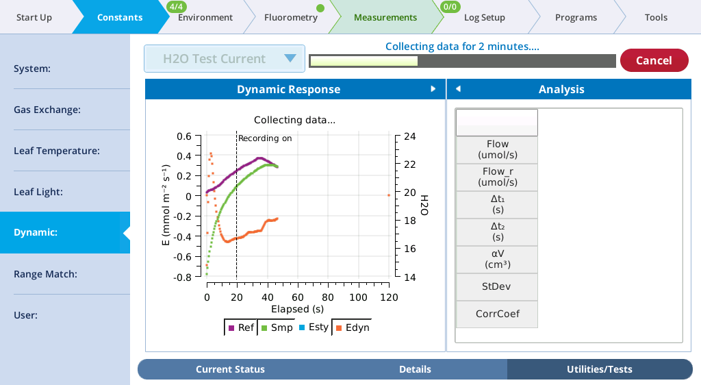
While data is being collected (Figure 9‑56), concentrations and fluxes are plotted on the real time graph, with the dynamic flux (Edyn) calculated using the current state of the Working table. Ideally, you'd want to see a minimum of variation in Edyn, and no correlation with whether the ramp is up or down. To put the Edyn behavior into perspective, tap the Esty graph legend button to also see the steady state flux plot.
When data collection is over (Figure 9‑57), standard deviation (StDev) and correlation with sample concentration (CorrCoeff) is computed for Edyn, and the results shown in the Before column of the table, along with the three fit parameters. A best fit routine is then run to find the values of the three tuning coefficients that minimize the variation about the mean, and those results displayed in the After column.
The "H2O Test Current" test prompts you for adding to the User table; the other test, "H2O Test Several" automatically adds them, but proves an option at the beginning to clear the User table.
Data collected during the test is stored in a file whose name and location depend on chamber model number, flow, and flow_r:
/home/licor/logs/dynamic/chamber/h2o/flow_flow_r.txt
For example, if you are using a 6800-01A chamber, have a flow of 600, and reference flow of 823, the file name would be
/home/licor/logs/dynamic/6800-01A/h2o/600_823.txt
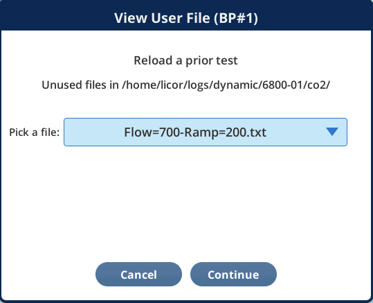
Reloading a test
The Utilities/Tests screen test options allow a previous test to be "reloaded". The opening dialog - in this case, for a CO2 test - presents a list of the files to choose from that are not already part of the User table.
If you select a file, it is read and plotted, and the resulting display will be just like the Test Current test (Figure 9‑54 for CO2 or Figure 9‑55 for H2O ).
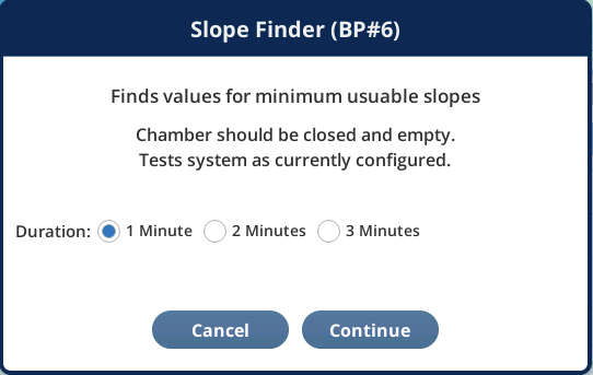
Measuring minimum usable slopes
The Slope Finder utility provides a method for setting an appropriate value for the minimum usable slopes. To run this test, set the controls for the desired CO2, H2O, flow, and fan settings you wish to test. The chamber should be empty and closed.
The test consists simply of recording rates of change of CO2 and H2O for some period of , and determining the maximum slope over time period (Figure 9‑59).
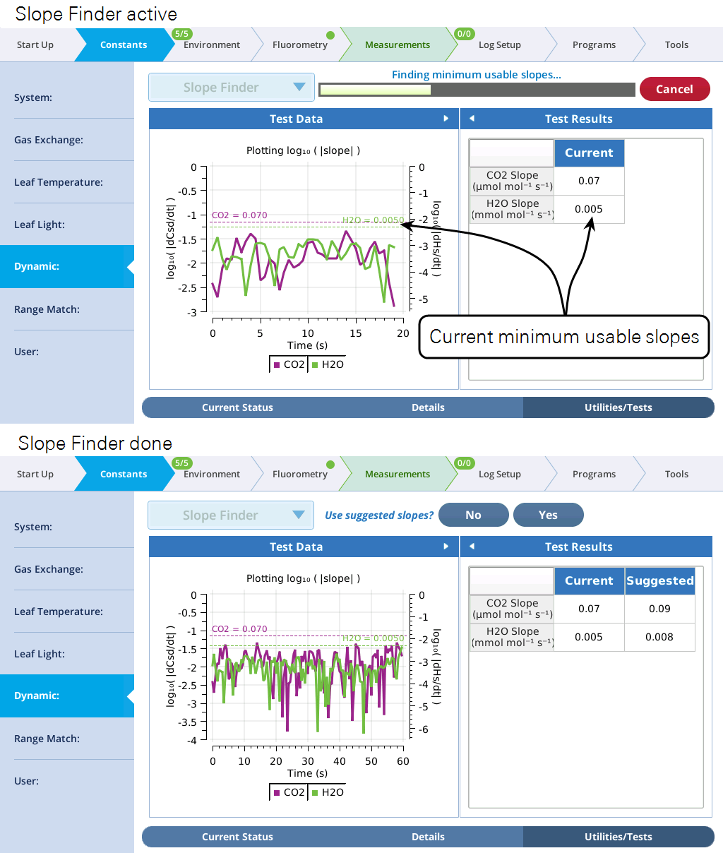
While the test runs, the graph plots the absolute value of the log of the slopes, and indicates the current value of the minimum usable slope (Figure 9‑60).
At the end of the test, you are given the chance to implement the suggested values, which are 2 times the measured maximum slopes.
Dynamic details
Equation derivation
The mass balance of water for air flowing through a single-volume, well mixed chamber is given by equation 9‑103:

| Symbol | Units (s) | Description |
|---|---|---|
| E | mol H2O m-2 s-1 | Transpiration rate |
| s | m-2 | Leaf area |
| ρ | mol m-3 | Air density |
| ue | mol s-1 | Flow of air entering chamber |
| uo | mol s-1 | Flow of air leaving chamber |
| v | m3 | Chamber volume |
| we | mol H2O (mol air)-1 | Water concentration entering chamber |
| wo | mol H2O (mol air)-1 | Water concentration leaving chamber |
Since uo = ue + sE, we can eliminate the unmeasured uo and rearrange to

For the mass balance of CO2 for air flowing through a single-volume, well mixed chamber, we eliminate the diluting effects of H2O by considering equivalent dry mole fractions cʹe and cʹo.
9‑105

| Symbol | Units (s) | Description |
|---|---|---|
| a′ | dry moles CO2 m-2 s-1 | Assimilation rate (dry equivalent) |
| a | mol CO2 m-2 s-1 | Assimilation rate |
| c′e | mol CO2 (mol dry air)-1 | Dry equivalent CO2 entering chamber |
| c′o | mol CO2 (mol dry air)-1 | Dry equivalent CO2 leaving chamber |
| ce | mol CO2 (mol air)-1 | CO2 entering chamber |
| co | mol CO2 (mol air)-1 | CO2 leaving chamber |

The equivalent dry mole fractions are
9‑107

Note that for steady state ( and
and  ), equation 9‑104 and equation 9‑106 reduce to the normal LI-6800 equations
9‑108

9‑109

Dynamic (non-steady state) transpiration is calculated in mmol m-2 s-1 by
9‑110

Non-steady state CO2 assimilation Adyn (µmol m-2 s-1) is given by:
9‑111

| Symbol | Units (s) | Description |
|---|---|---|
| Adyn | µmol CO2 m-2 s-1 | Assimilation rate |
| Crd | µmol CO2 (mol dry air)-1 | Equivalent dry reference concentration |
| Csd | µmol CO2 (mol dry air)-1 | Equivalent dry sample concentration |
| Edyn | mmol H2O m-2 s-1 | Transpiration rate |
| F | µmol s-1 | Flow entering the chamber |
| P | kPa | Chamber atmospheric pressure |
| T | C | Chamber air temperature |
| V | cm3 | Relevant volume |
| Wr | mmol H2O (mol air)-1 | Reference water concentration |
| Ws | mmol H2O (mol air)-1 | Sample water concentration |
Three tuning parameters
On the LI-6800, the dynamic equations have three parameters Δt1, Δt2, and αV that can be tuned for optimum accuracy, empirically making up for all the differences between the idealized system for which the equation is derived, and the actual system on which it is implemented. Consider CO2: the heart of the equation contains a reference reading, a sample reading, an effective volume, and a slope.
9‑112

Δt1 is the time offset to use for the reference concentration. For example, if Δt1 = 1.2, the value for Crd would be an interpolated value coming from 1.2 seconds before the Csd sample value. Similarly, Δt2 is the time offset at which the sample slope is computed. αV is an empirically determined "volume" that provides the best fit.
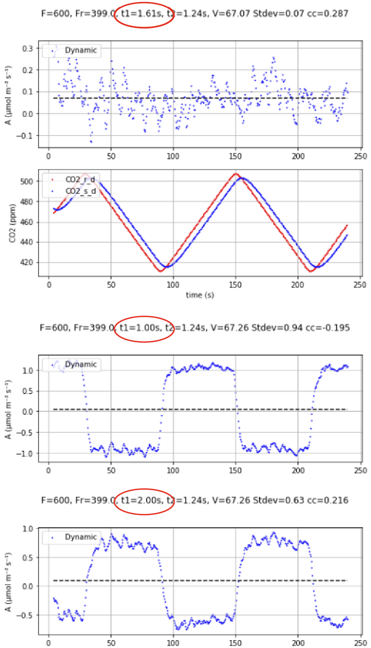
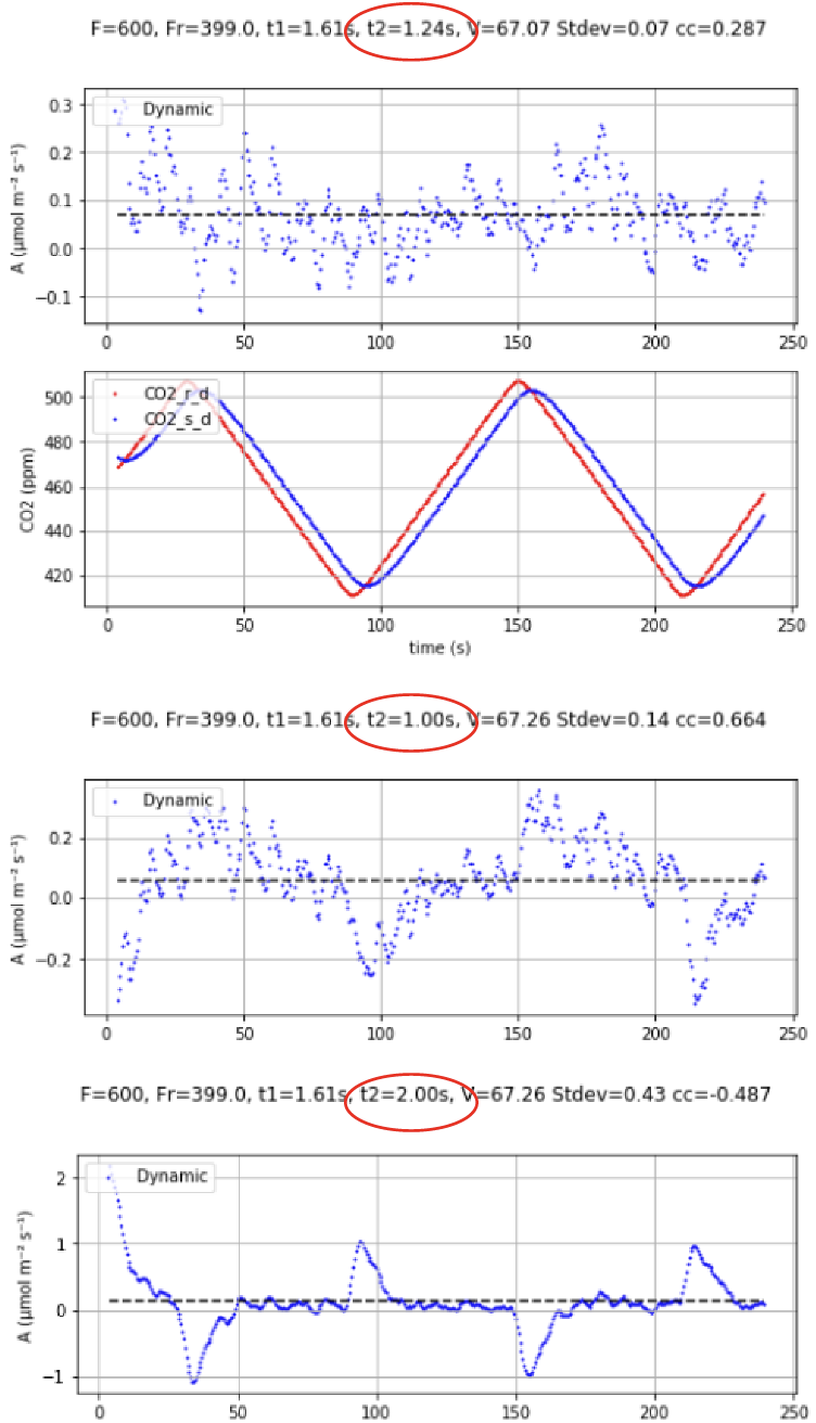
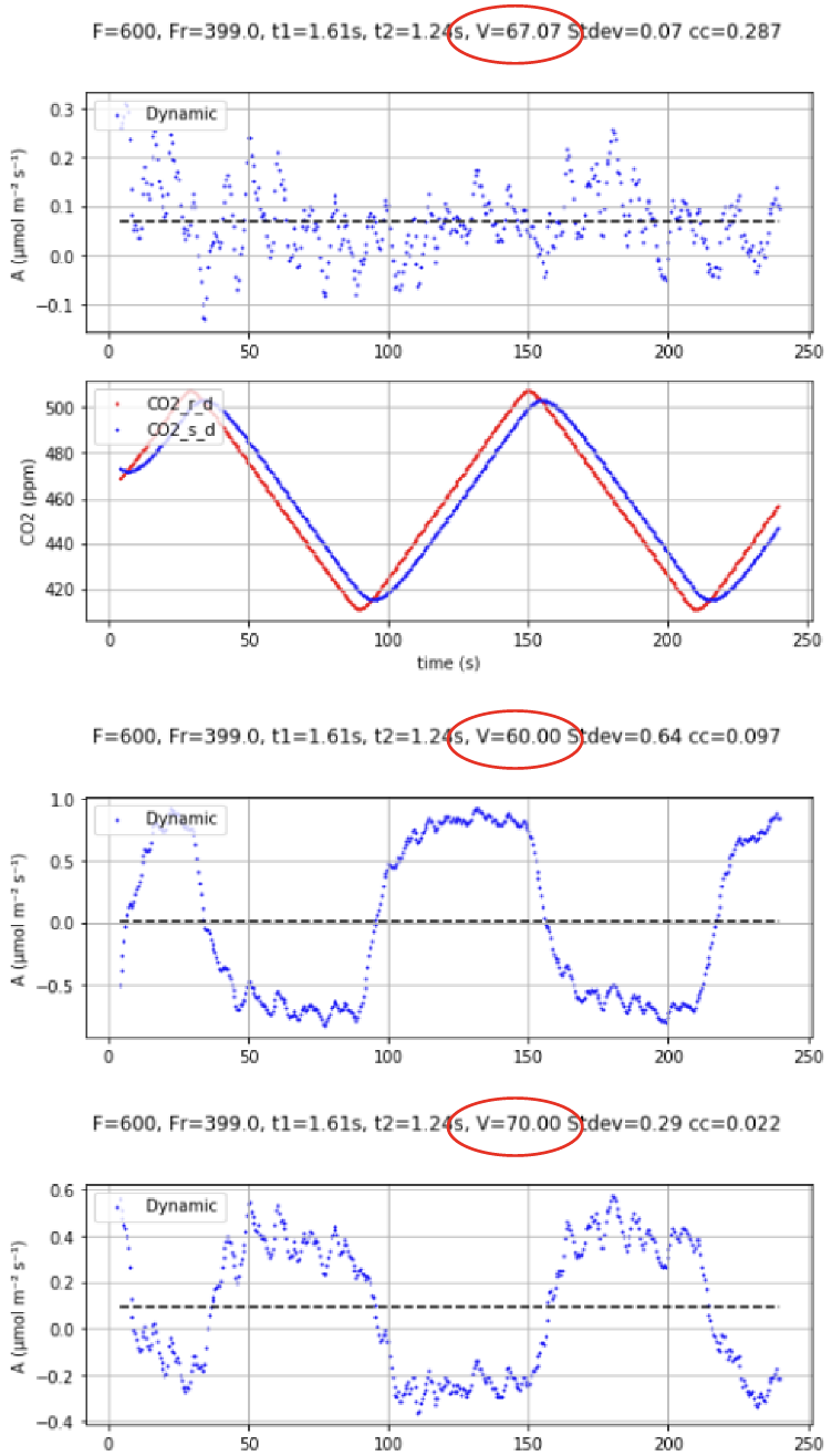
Implementing the dynamic equations involves keeping a running buffer of data so that, for any value of Csd, we can get a Crd from some Δt1 prior, and a dDsd/dt computed from the Csd data stream at some Δt2 prior. Figure 9‑61 and Figure 9‑62 illustrate.
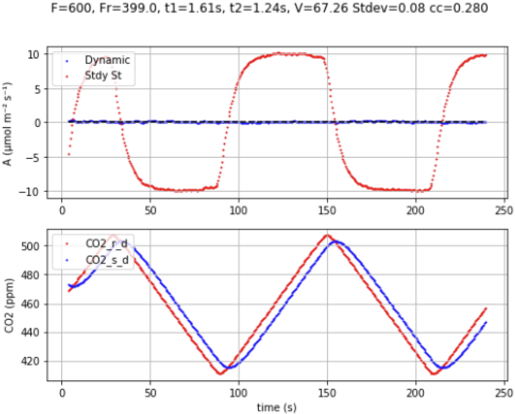
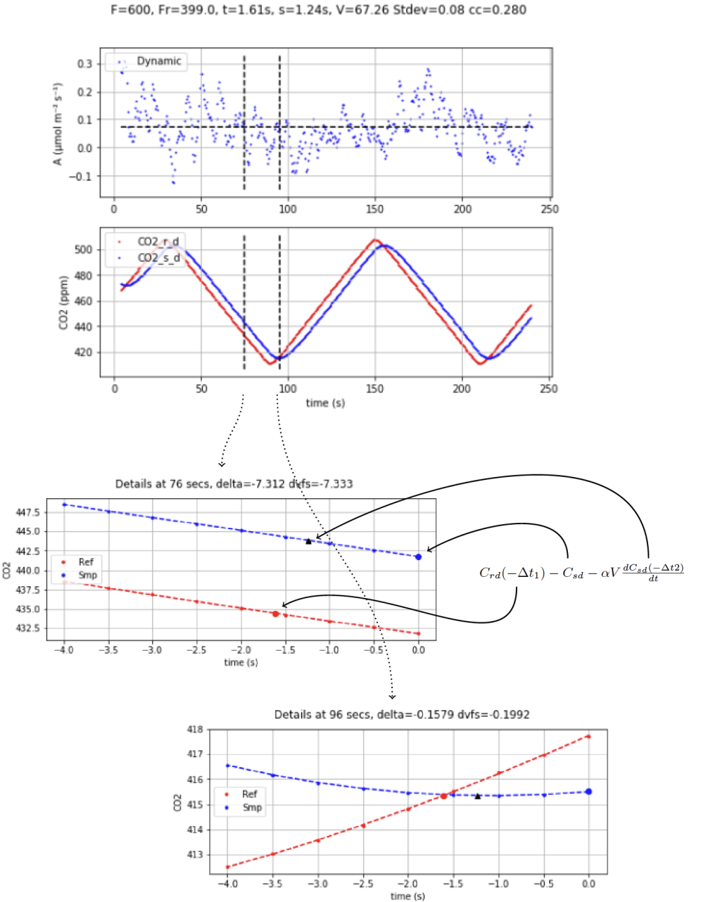
Figure 9‑63 illustrates how varying Δt1 changes the computed value of Adyn for an empty chamber saw-toothed experiment, where the known flux is 0. Similarly, Figure 9‑64 shows the effect of Δt2, and Figure 9‑65 illustrates the effect of αV.