Theory and equation summary

Carbon dioxide in soil is primarily produced by root respiration, decay of organic matter, and activity of microbes. Rainwater can have direct effects as well, by displacing gas in soil pore spaces, and by interacting with limestone soils. Also, rainwater itself carries some dissolved CO₂ that can be released in the soil.

Thus, soil CO₂ flux is dependent on soil temperature, organic content, moisture content and precipitation, and has a great deal of spatial variability. Soil CO₂ flux is also extremely sensitive to pressure fluctuations. An unvented chamber will induce significant pressure increases just by closing. Soil water evaporation and heating of the air in the chamber head space also induce pressure increases in an unvented chamber. The LI-6800 Soil CO₂ Flux Chamber is vented so that pressures inside and outside the chamber are in a dynamic equilibrium.

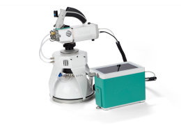
The chamber is designed to mitigate factors that can induce variation in measurements with the following features:

• A bellows-controlled closure mechanism, which ensures that placement of the chamber has the same negligible effect with each measurement sample.
• A patented chamber vent that maintains ambient pressure inside the chamber, even in windy conditions.
• Soil collars, which, after installation, ensure consistency between samples.

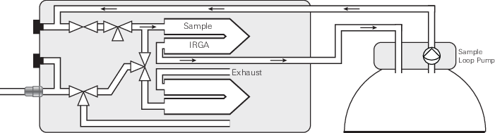
In contrast with the LI-6800 leaf chambers, which are an open gas exchange system, the soil CO₂ flux chamber is a closed system. Instead of sample and reference gas analyzers, the LI-6800 uses the sample IRGA in this configuration. Instead of using the console flow pump, the soil chamber has its own circulation pump. When the chamber is closed, the chamber pump circulates air through the sample analyzer exhaust to the chamber and then back to the sample analyzer (see Figure 11‑1).

The measurement cycle

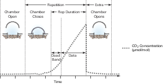
When the chamber is placed on a soil collar it will remain open until the measurement is started. When the measurement is started, the bellows pump closes the chamber. Upon closing, the instrument begins logging data, and the dead band starts (see Figure 11‑2). The instrument continues to record data for the duration of the repetition, and then the chamber opens and pauses for the extra duration. The measurement repeats for the specified number of repetitions.

Equation summary

Soil CO₂ flux (F) is computed with the following equation:

11‑1

where V is chamber volume (cm³), P is atmospheric pressure (kPa), W is the water mole fraction in the chamber (mmol mol^-1), R is the gas constant (8.314 J K^-1 mol ^‑1), S is the exposed soil area (cm²), T is chamber air temperature (°C), and C' is dry CO₂ concentration (mol mol ^-1), given by:

11‑2

Since the measurement occurs in a closed system, C' increases with time, reducing the carbon dioxide gradient between the chamber and the soil beneath, which in turn reduces the flux. Since CO₂ is diffusing from the soil into a closed volume, we make the assumption that the relationship between C' and time is:

11‑3

The rate of change (C') with time is then:

11‑4

We want to compute the flux at the time (t_o) the chamber closed (and C'(t_o) = C'_o), so we need corresponding initial values of T, P, W. These are determined by fitting a straight line to the first 10 seconds of data once the chamber closes, and computing the intercept value. The initial rate of change comes from equation 11‑4 evaluated at t_o.

11‑5

F_o, the flux at t = t_o, is thus:

11‑6

and flux (F_target) at any other target concentration (near C'_o) can be computed by solving equation 11‑3 for t such that C' = C'_target:

11‑7

then using t_target in equation 11‑4 to compute the appropriate rate of change.

The constants C_x and a in equation 11‑4 come from curve fitting equation 11‑3, which requires non-linear regression. During a measurement, and before the actual curve t, we can estimate F_o by noting the following: if we fit a line to plotted against C', we can use its slope and intercept to get an estimate of a and C'_x. This relation comes from eliminating the exponential from equation 11‑4 using equation 11‑3:

11‑8

Thus, a is the negative of the slope of such a plot, and C_x is the intercept value divided by a.