What's new in version 2.1

This document summarizes changes in the latest version of Bluestem OS for the LI-6800 Portable Photosynthesis System. Review this if you are familiar with older versions of the software and you want to learn what is new.

Stevens HydraProbe options

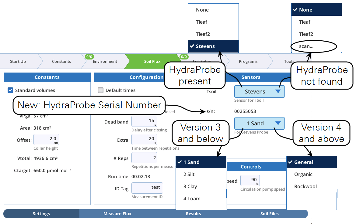
This update supports the newer versions of the Stevens HydraProbe used with the Soil Respiration chamber. HydraProbes with firmware version 4.0 and above have different options for soil type / calibration media. The minor interface changes to the LI-6800 are described in Figure 1.

The following summarizes expected behavior:

1. If a HydraProbe probe is attached when the soil chamber configuration is enabled:
   1. T_soil will automatically be set to Stevens, regardless of its last setting.
2. If a HydraProbe is not attached when the soil chamber configuration is enabled:
   1. T_soil will show the last setting, or None if the last-time setting was Stevens.
   2. The T_soil menu will include scan.... Selecting scan... will (if a probe has been subsequently attached) find and enable the probe. (You might have to wait up to a minute after attaching the probe for scan... to work. If scan... doesn't immediately  find the probe, wait a bit and try it again. If all else fails, change the system configuration away from the soil chamber and back again.)
3. The s/n (probe serial number) and Soil Type entries are "—" if a probe is not active (T_soil not set to Stevens).
4. Soil Type will return to its previous value if you change from Stevens to something else, and back again, or from one session to the next. However, if the HydraProbe itself changes, and crosses the version 3 boundary, Soil Type will default to 1 Sand (version 3 or below) or General (version 4 and above).

Miscellaneous changes

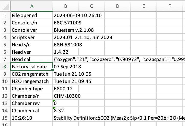
Factory calibration date

The factory calibration date has been added to log  file headers (see ).

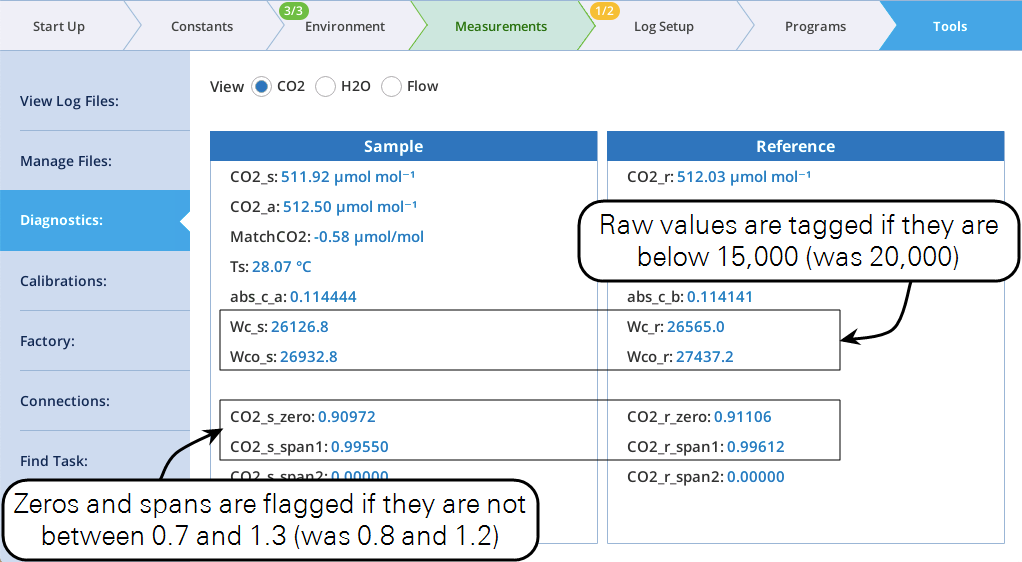
W

Flagging criteria loosened

Criteria for flagging warnings in the CO₂ and H₂O IRGA diagnostics pages have been loosened.

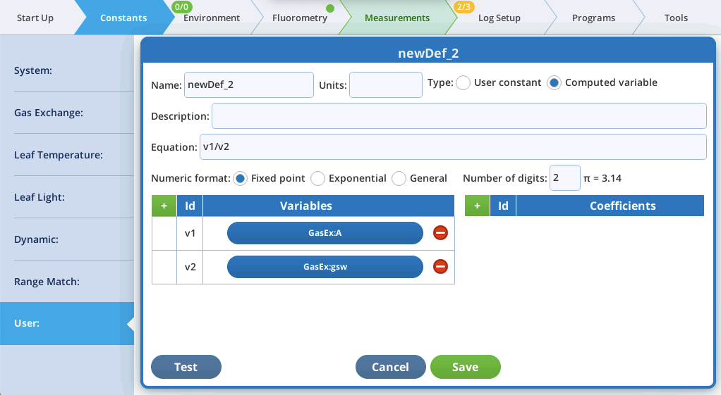
User-defined equations

Version 2.1 supports a number of math functions (Table 1) that can be used when specifying an equation for a user-defined variable that will carry over to the Excel spreadsheet version of the log file.

Table 1. Python methods that can be used in a user-defined variable, and how they appear in the Excel log file.

Python	Becomes in Excel
math.ceil(x)	CEILING(x,1)
math.cos(x)	COS(x)
math.degrees(x)	DEGREES(x)
math.e	EXP(1)
math.exp(x)	EXP(x)
math.fabs(x)	ABS(x)
math.log(x)	LOG(x ,EXP(1))
math.log10(x)	LOG10(x)
math.pi	PI()
pow(x,y)	POWER(x,y)
math.radians(x)	RADIANS(x)
math.sin(x)	SIN(x)
math.sqrt(x)	SQRT(x)
math.tan(x)	TAN(x)

Daily automatic snapshots

Version 2.1 will take one daily snapshot automatically after the system has been on (and not sleeping) for at least one hour. These automatic snapshots contain a subset of a manually generated snapshot, since the focus is on the system hardware. They can prove useful later when troubleshooting, such as determining when some issue started to appear.

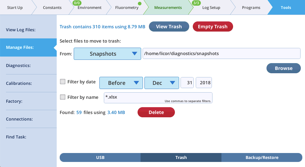
Automatic snapshots are typically 50K bytes in size. If disk space becomes a consideration, use the Tools > Manage Files > Trash utility to see how much space is being used by snapshots (or log files, etc.), and to easily move unneeded files to the trash. (File space is not reclaimed until the trash is emptied.)

Summary of fluorometry changes

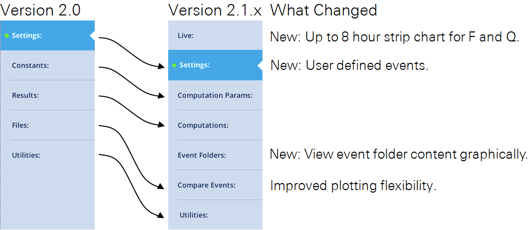
Tab names

The Fluorometry tabs have a new look, with two additions and several name changes.

Modulation is On automatically

In version 2.1 the modulation beam will be turned ON (if it is Off) automatically in the following circumstances:

• Opening a log file.
• Triggering a fluorescence event, manually or via log.
• Turning fluorescence recording on or off.

For most users, this change represents a certain degree of insurance against inadvertently logging data with the measuring beam off (which renders all modulated fluorescence values invalid.) A note of caution, however: the Fo (or Fo′ ) value that is logged is based an averaged modulated F (averaging time set in Fluorometry > Settings > Measuring). If you turn off the measuring beam and log or otherwise trigger a flash, the measuring beam will come back on, but averaged F value will be near 0, since the modulation was only just turned on.

If you actually wish to log fluorescence events with no modulation, then the way to achieve that is by setting the modulation setpoint to zero (also in Fluorometry > Settings > Measuring). This effectively keeps the modulation LEDs off when the modulation is set to “ON”.

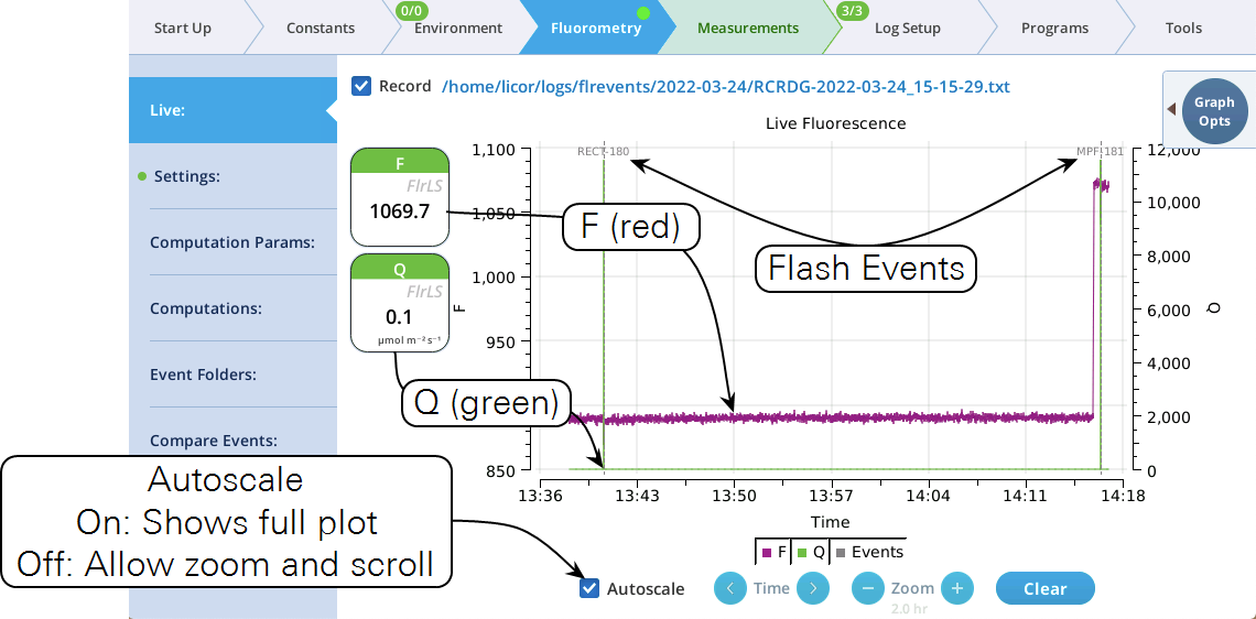
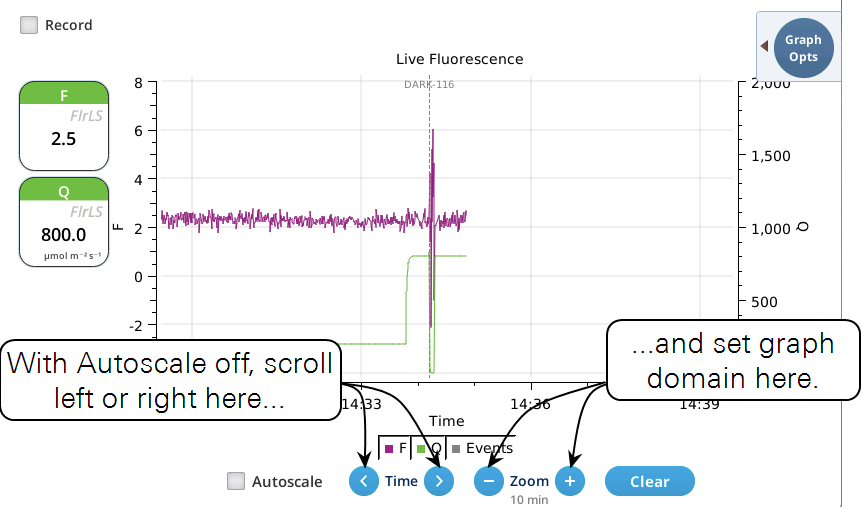
Live

Version 2.1 adds a Live screen for monitoring fluorescence. The graph uses a time-of-day bottom axis, and plots modulated fluorescence F and actinic light Q for up to 8 hours. Fluorescence events (saturating flashes, dark pulses) are also marked on this graph as they happen.

Operational tips:

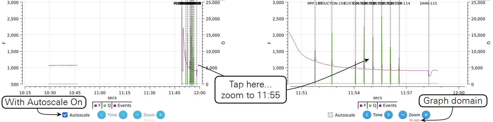
• While the Autoscale box is checked, you can quickly zoom in on a part of the graph by simply tapping the graph at that location. The graph will automatically turn Autoscale off and center itself at the tapped time, with the range of the displayed data set by the current Zoom setting. Subsequent left/right shifting and zooming in/out is done by the Time and Zoom buttons. To get back to the full view, check the Autoscale box.



• While Autoscale is unchecked, the graph will remain unchanged if the newest incoming data is not on screen. If the present time is visible, the graph will automatically scroll left each time the incoming data reaches the right edge, keeping the latest x minutes (x = whatever the zoom is set to) visible on screen.



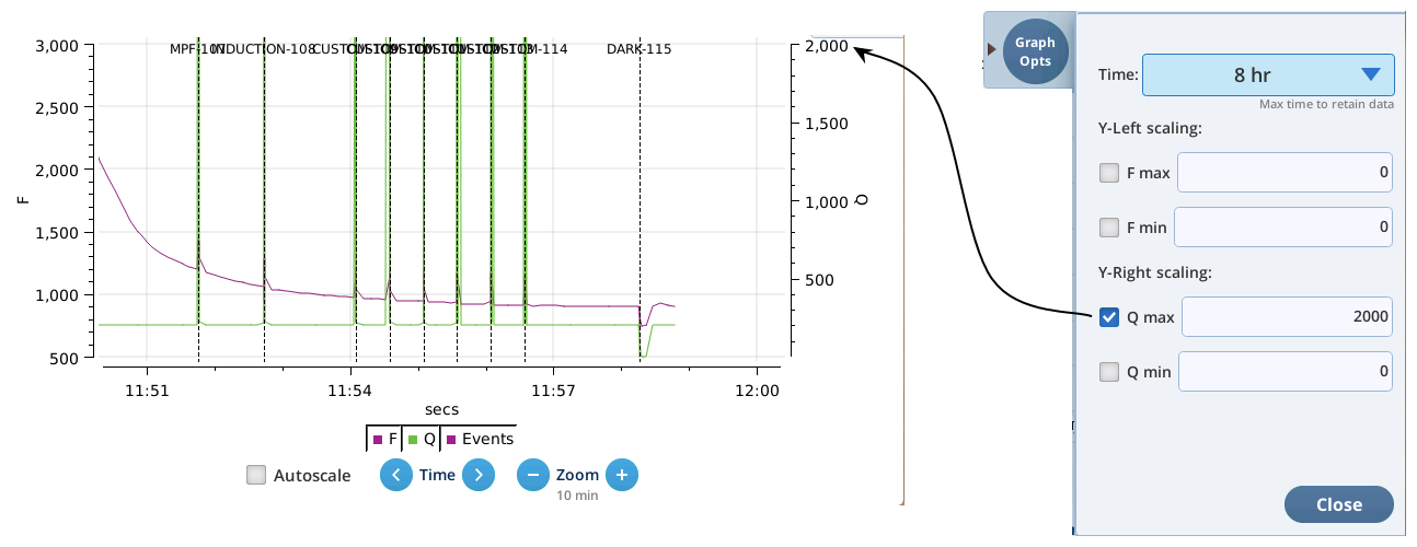
• The Q plot is easily dominated by saturating flashes (e.g., max values of 15,000). To maintain a normal actinic scale, open the Graph Opts panel, set Q max to 2000 and check the Q max box.



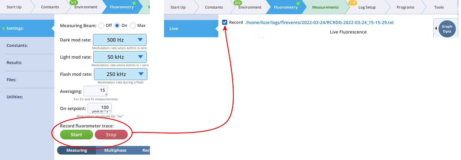
• The Record checkbox replaces the Start/Stop buttons that used to reside on the Measuring Settings page (Figure 10). Record has no influence on the real-time graph, which keeps going no matter what (unless you put the instrument to sleep).

A fluorescence trace file contains tab-delimited records of 9 fluorometer output values. The first line is always a label line.

Event folders

The Event Folders screen represents a graphical way to explore the contents of /home/user/logs/flrevents, which holds daily directories of fluorescence events and recording files. A date/folder picker allows the user to pick the daily folder to be viewed. A label indicates how many recording or events files are found there, and a Plot button causes the contents of the directory to be read and displayed on the graph.

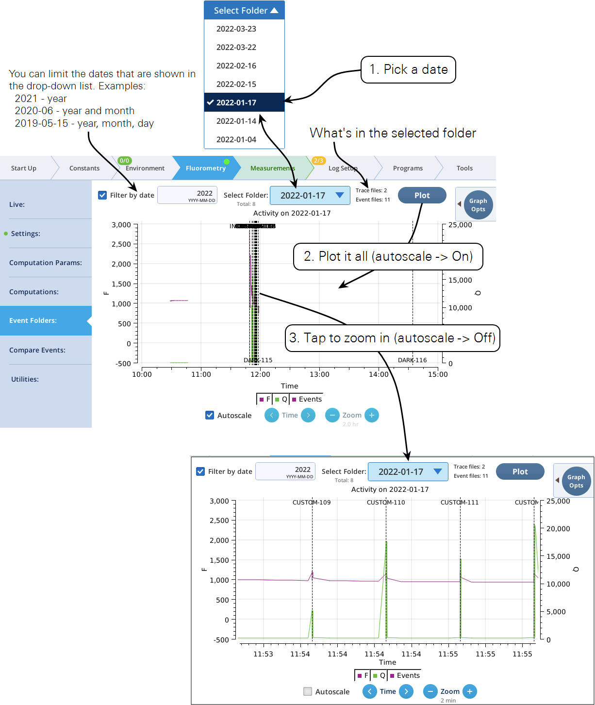
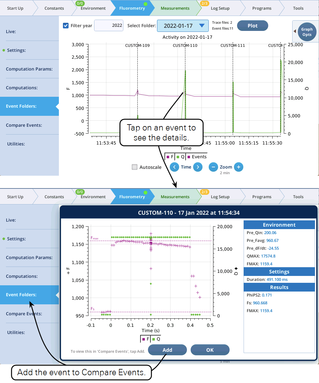
With Autoscale off, tapping the graph close to an event will open a dialog with a plot of the event and related details (Figure 12). If this event is not already in the list of events in Compare Events, you can add it simply by tapping the Add button in the dialog. (If it is already there, no Add button will be displayed.)

Settings > Custom

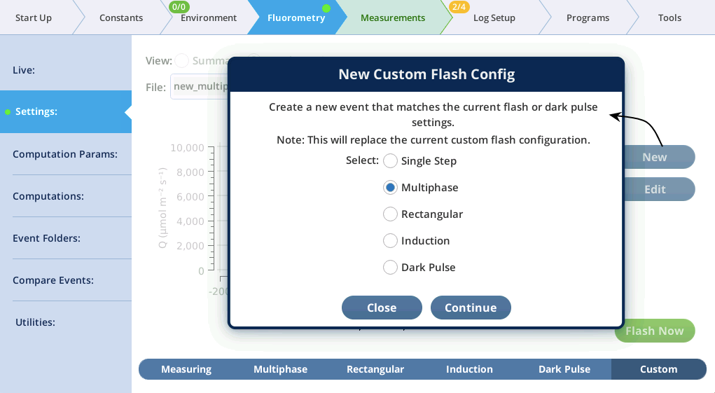
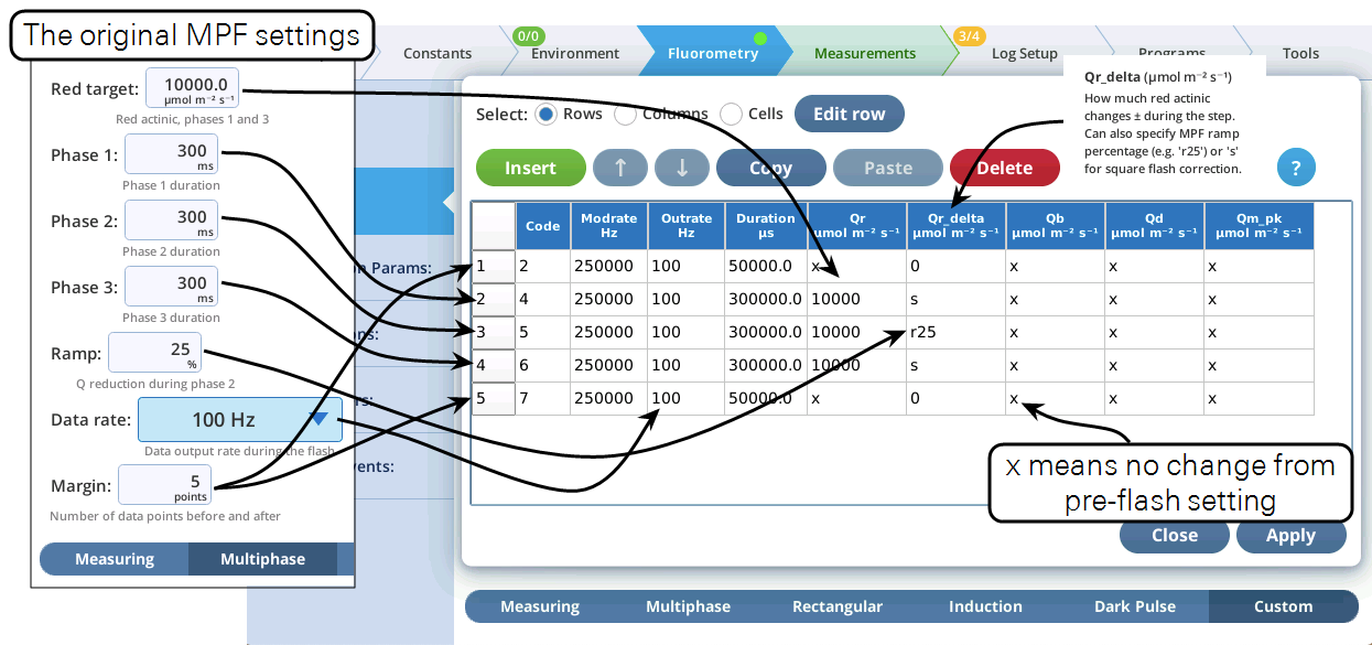
LI-6800 Software version 2.1 (and fluorometer/head firmware version 1.4.21 and higher) supports a user-defined custom flash. With this new feature, you can define up to 38 steps to be executed during a flash, and in each step specify duration, modulation rate, output rate, intensities of red, blue far red, modulation beam peak intensity, and rate of change of red actinic intensity. (We’ve called this a “flash”, but more generally this is an event, since it could be a dark pulse, or flash and a dark pulse, or anything you’d care to define.)

For a quick introduction, here is a brief tour, in which we’ll make a custom flash that will combine an MPF and a Dark Pulse into one event.

1. In the Settings > Custom screen, tap New, pick Multiphase, and tap Continue (Figure 13).



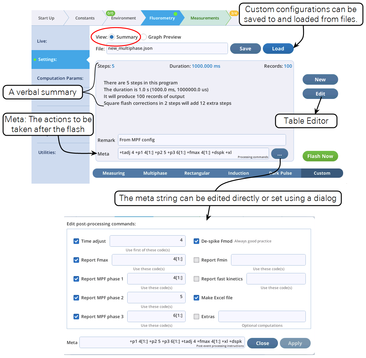
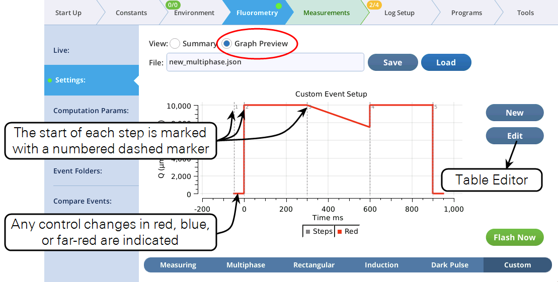
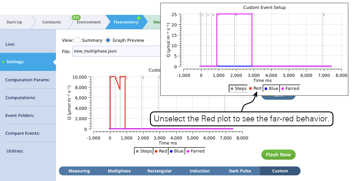
2. The Settings > Custom screen provides three views of the custom flash: text summary (Figure 14), a graphical preview (Figure 15), and an editable table (Figure 16).







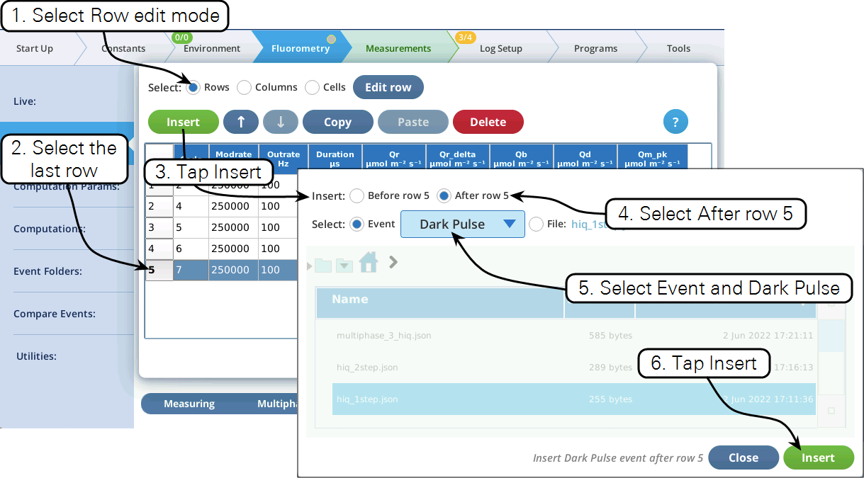
3. Now let's modify this event by adding a dark pulse to the end of it to measure Fo' all in one event. Go to the Table view, be sure you are in Row edit mode, tap row 5 to select it, then tap Insert (Figure 17).



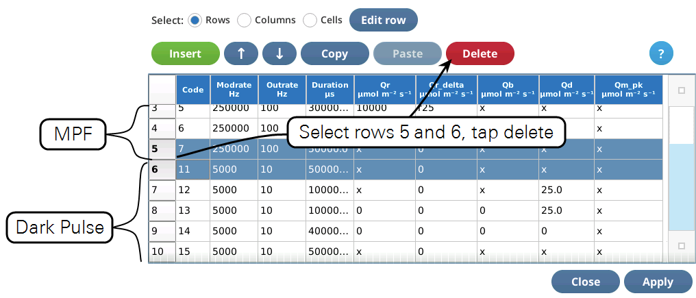
4. Once the two events are merged, we have to get rid of the final margin for the MPF (row 5, Code is 7), and the starting margin step for the Dark pulse (row 6, Code is 11). To do this, select them both (tap on row 5, drag down to row 6) and tap1 Note: we could also get rid of these two steps by setting the Duration value for rows 5 and 6 to 0, since 0 duration steps are simply skipped.Delete (Figure 18). Then tap Apply to keep the changes you made.



5. The graphical preview shows a combined MPF and dark pulse event (Figure 19).



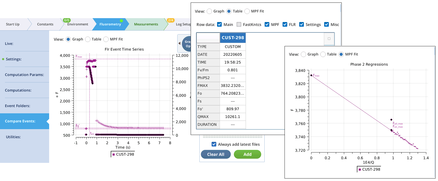
6. Test the custom event by tapping Flash Now , and examining the results in the Compare Events screen (Figure 20).

Compare events

Graph view

The Fluorometry > Compare Events section has some changes to better support viewing fluorometer event files.

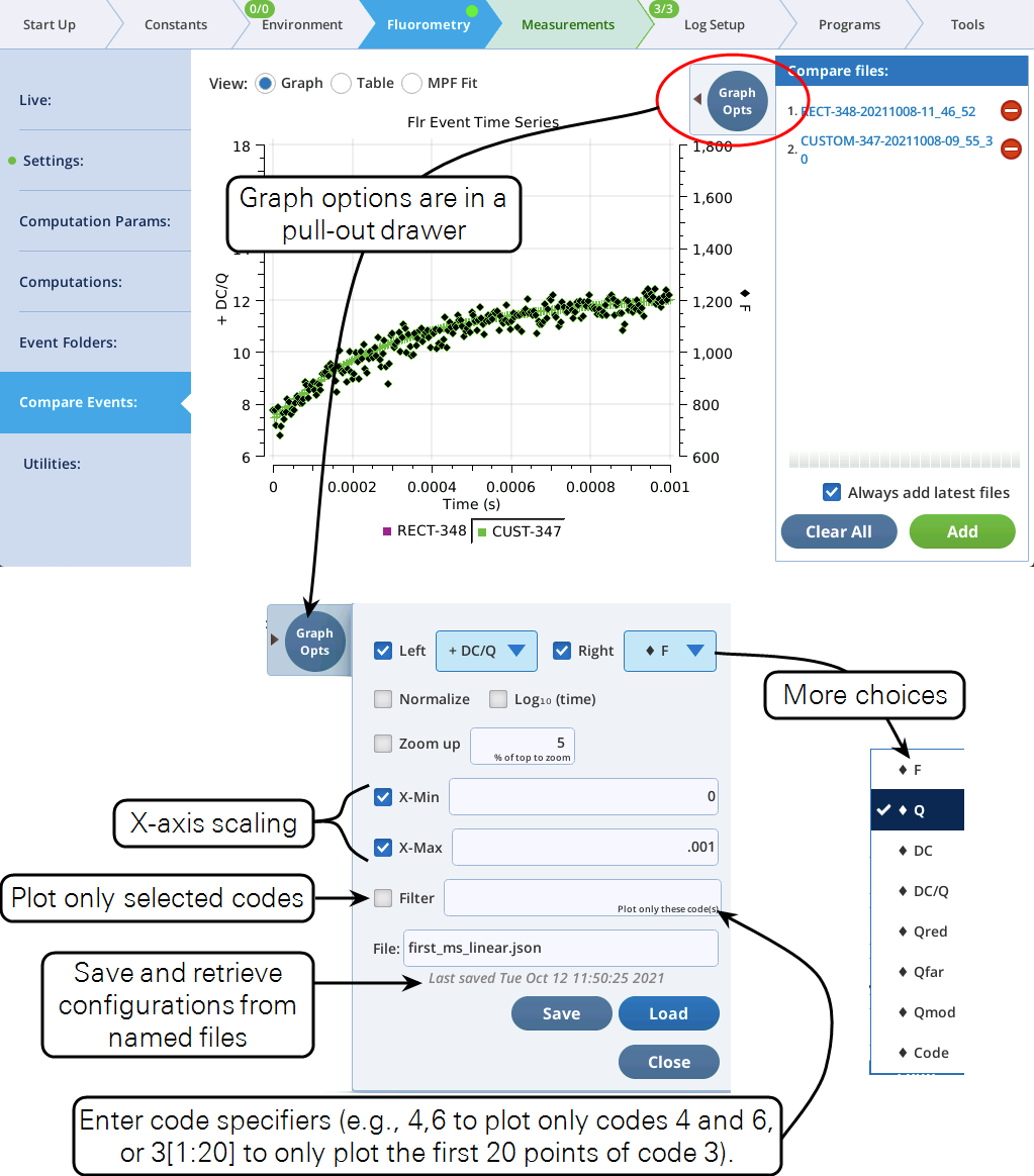
Using codes

The Filter field in Figure 21 also allows you to specify parts of a flash event to graph. For example, to see a RECT flash without the margin points, specify 3. To plot just the first and third phases on an MPF, specify 4,6. Table 2 shows code value usage.

Table 2. Step code usage.

Code	Description
2	Pre-flash margin
3	RECT or INDUCTION flash
4	MPF Phase 1
5	MPF Phase 2
6	MPF Phase 3
7	Post-flash margin
8 - 10	unused
11	DARK pre margin
12	DARK part 1
13	DARK part 2
14	DARK part 3
15	DARK post margin
16 - 53	CUSTOM

Code number(s) represent a list of indices. For example, consider a hypothetical flash data set that includes these time series data:

Suppose the filter code is 17. This means the plot will be of data whose 0-based indices (potentially 0 thru 9) are where CODE is 17. The list of indices where this condition is true is

so whatever is being plotted, it will be only those indices.

Code specifiers can include slice information (using the Python slicing convention), allowing you to further filter the list of indices. The syntax is (no spaces!)

where code is the code number, start is starting index, defaults to 0, stop is stopping index, defaults to None, and step is the step count, defaults to 1. start and stop can be positive (count from the left end) or negative (count from the right end).

Examples using the above hypothetical flash data are shown in Table 3.

Table 3. Code specifier examples and results.

Specifier	Resulting Indicies	Description
16,17,18	[0, 1, 2, 3, 4, 5, 6, 7, 8, 9]	Use just those three codes
17	[2, 3, 4, 5, 6]	All code 17s
17[1:]	[3, 4, 5, 6]	Skip the first one
17[:-2]	[2, 3, 4]	Skip the last 2
17[0:4]	[2, 3, 4, 5]	Use only the first 4
17[::2]	[2, 4, 6]	Use every other one
16[0],18[-1]	[0, 9]	Use first of 16, last of 18

Table view

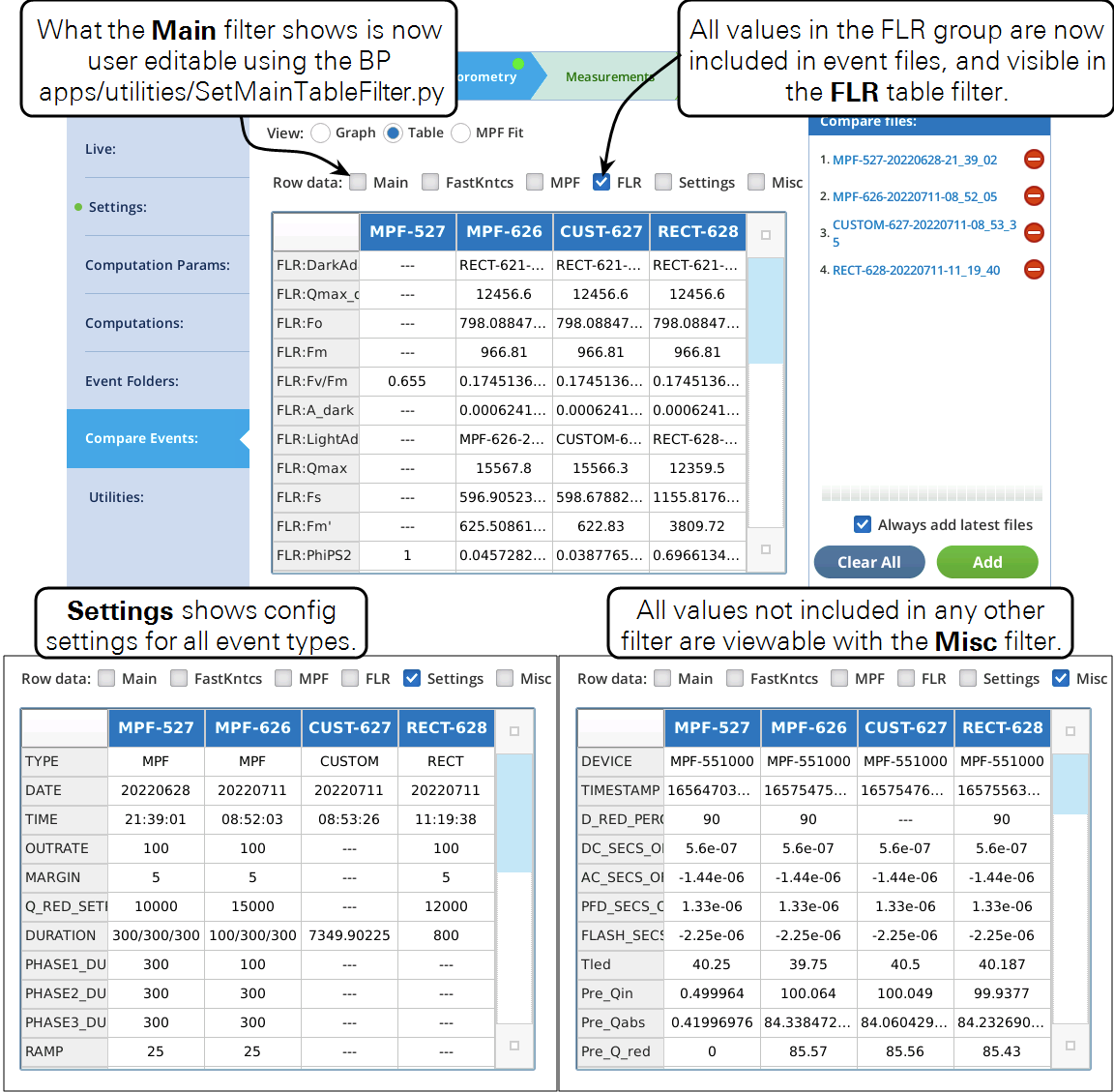
The Table view has a couple of enhancements (Figure 22).

Fluorometer file changes

The addition of custom flash events has caused some minor changes to the fluorometer event file structure. These changes will not impact most users, except those who analyze event files with their own software.

Listing 1 shows the .json file for a standard rectangular flash. The red sections of the header, and the in the computations, depend on event type. The green section is new, and contains all of the FLR group values following this event).

Listing 1. A standard rectangular flash. The red highlighted sections will change with event TYPE.

Fluorometry timing details

The relative timing of the modulation, various measurements, and actinic change ("Saturating Flash") is shown in (Figure 23).

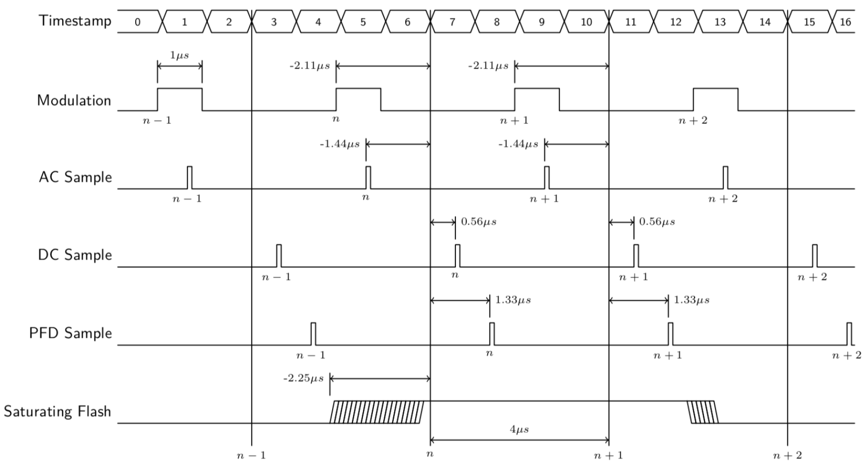
The vertical lines marked n- 1, n, etc. represent data output at a common time stamp. The measurements made associated with that stamp differ slightly from the actual time stamp by small amounts. For example, the PFD (actinic) measurement is made 1.33 µs after the reported time, while the modulated fluorescence is measured 1.44 µs prior to the reported time. These offset values appear in each ash event file, so any firmware updates that change timing will be documented in the fluorometer's output (Listing 2).

Listing 2. Timing information.