Measuring Small Volumes of CO₂

In some gas exchange applications, only a small volume of gas (5 ml or less) is available for measurement (as when measuring the respiration of insects or a single fruit, for example). Because this volume is too small to flow through the LI-7000 in a normal fashion, CO₂ concentrations must be measured by a different technique.

A small sample volume is drawn into a syringe and injected into a CO₂-free air stream that is flowing through the B cell (sample cell). A calibration curve must be generated first by measuring one or more known gasses. By selecting the proper injection volumes and flow rates a wide range of CO₂ concentrations can be measured. CO₂-free air should be entered into cell A (reference cell). This can be accomplished by using either a tank of certified CO₂-free air, or by scrubbing the incoming air with a column of soda lime.

The sample air stream should also be free of CO₂ prior to the sample injection. Again, you can use either a tank of CO₂-free air, or you can pump air through a column of soda lime. Insert a short piece of gum rubber tubing into the sample stream just before the entrance to the sample cell. This will be your injection point. Be sure to minimize the length of this gum tubing, as some CO₂ diffusion is likely to occur here. Alternately, you can replace this piece of gum rubber tubing with a T-fitting. You can insert a septum in the T-fitting, and inject your samples through this septum. The septum should not allow as much diffusion as the gum rubber tubing.

When your system is set up, you will want to zero and span the LI-7000, using flow rates similar to those that you will use during your experiment. Flow rates at or below 2 liters per minute work well for this type of work.

Configure the LI-7000 to display channels 30 and 31. Channel 30 is the integration result, area under the curve. Channel 31 is the integration result peak value. Set your instrument to integrate the CO₂B channel either automatically with threshold values or manually.

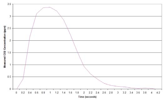
You are now ready to generate your calibration curve. This curve is established by plotting either the integral of the CO₂ with respect to time against the known concentration, or by plotting the integration peak value against the known concentration. The LI-7000 provides you with instantaneous readout of both the integrated value and the peak height. Figure 1‑1 shows a typical injection curve, using a sample flow rate of 0.5 liters per minute, and injecting 1 cc of 377 ppm CO₂.

Draw a known concentration of CO₂ into a syringe. It is a good idea to over fill the syringe slightly, and expel a small amount just prior to making your injection.

If you are manually starting and stopping the integration, you will want to start it just prior to your injection. Then inject your sample, and wait for the instrument to flush out all of the CO₂ from the sample cell. It is important to inject your samples at a consistent rate. You may require some practice to perfect your injection technique. It is easier to inject at a constant rate if you are working with smaller volumes (i.e., 1 ml rather than 5 ml).

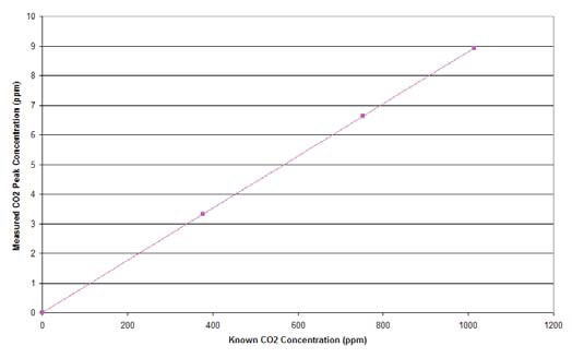
When you have constructed your flow rate and sample volume specific calibration curve you can use it to determine actual concentrations of unknown samples. Your calibration curve should be linear. Any non-linearity is likely due to inconsistency in injection rates or volumes. Figure 1‑2 shows a calibration curve generated from three known concentrations of CO₂.

Using this injection method with small volumes of CO₂, you can analyze concentrations of CO₂ that are much higher than the standard 0-3000 ppm calibration range. Concentrations of over 34,000 ppm can be analyzed when injected in volumes of 1 ml with sample flow rates of 0.5 Liters per minute. If using microliter sample volumes (up to about 35 μL), you can analyze pure CO₂.