Mapping CO2 Concentrations and Fluxes with the LI-8100A
Printable PDF: Mapping CO2 Concentrations and Fluxes with the LI-8100A
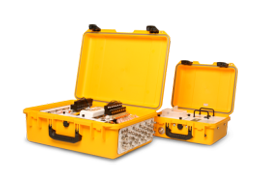
Instructions for the mapping kit.
The 8100-405 CO2 Mapping Kit is designed to interface with the LI-8100A Soil CO2 Flux System to allow spatial data to be integrated with observations of soil CO2 concentration.

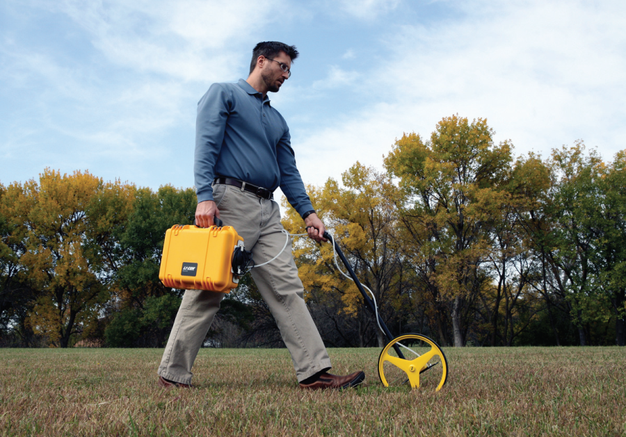
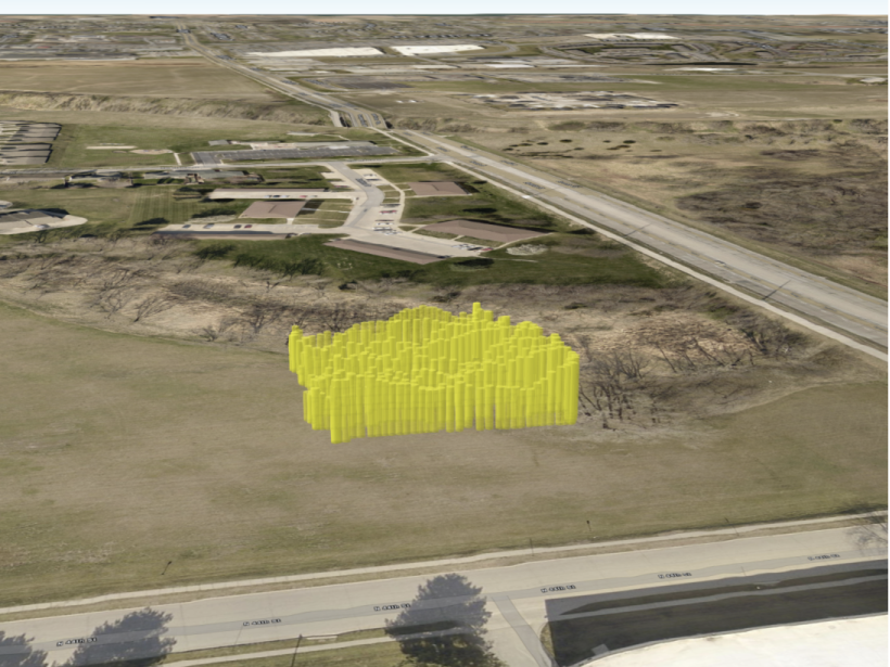
The mapping kit can be used with either of the instrument’s survey chambers (8100-102 and 8100-103) to map soil CO2 flux across a given area (Figure 1), or it can be used with the LI-8100A in continuous mode without a chamber to rapidly map CO2 concentrations (Figure 2).
Considerations for Concentration Mapping
Concentration mapping with the LI-8100A system requires a user provided intake tube from the sampling point to the Air In port on the side panel of the LI-8100A Analyzer Control Unit. Bev-a-line tubing and stainless steel quick-connect fittings are provided with the kit for constructing an intake tube, or to connect the instrument to existing sampling hardware. The design of the intake tube should be driven by the application.
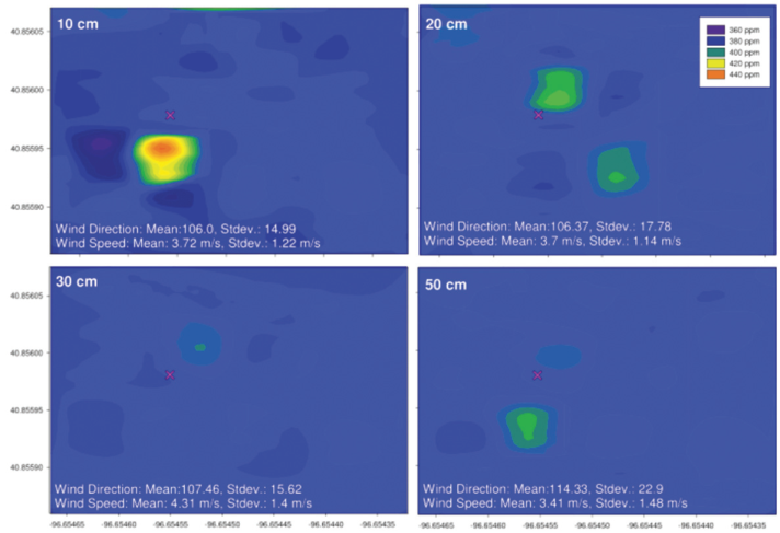
For leak detection, sampling height is a key consideration. In this application the instrument is used to detect potentially small plumes of CO2 from the ground, which under turbulent conditions mix readily with the atmosphere. The best way to detect these plumes is by sampling as close to the source as possible, which means the intake needs to be held close to the ground and at a constant height. As turbulence and measurement height increase the plume mixes more quickly with the bulk atmosphere causing CO2 concentrations to more rapidly approach background levels. Figure 3 shows an example data set where a small controlled release of pure CO2 was performed, and CO2 concentrations were measured at four fixed heights above the release point.
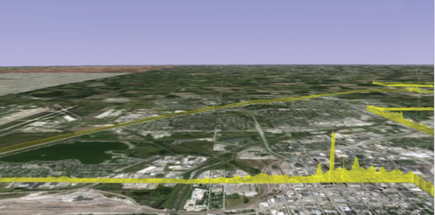
Data collected by the LI-8100A system for concentration mapping are formatted differently than data collected for soil flux measurements. In version 4.x of the LI-8100A instrument (embedded) software a continuous data collection mode was added. This mode allows the instrument to continuously record data for up to 24 hours after a measurement is started. The data exclude the headers and footers included in the standard .81x data file, and are formatted as comma delimited text. Data collected in continuous mode can be formatted for display in Google® Earth using the KML converter application installed with the LI-8100A Windows® application software.
The KML converter supports export of any variable included in the file to an extruded track, where elevation of the track above ground is directly proportional to the measured value (example shown in Figure 2). It also allows export of file annotations as placemarks in a separate .kml file. A short guide to exporting data collected in continuous mode to Google Earth is given below. To configure the instrument for continuous measurements please refer to the 8100-405 instruction manual.
Exporting Data for use in Google Earth
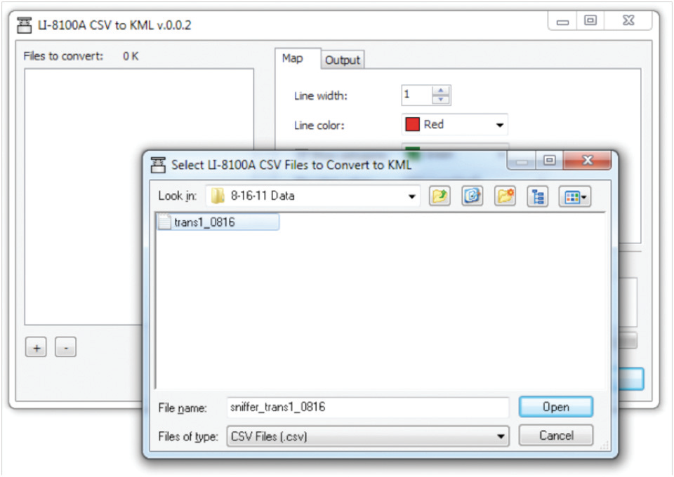
To export data from .csv files collected in continuous measurement mode, move the files from the LI-8100A to the host computer and launch the LI-8100A CSV to KML converter program. Click the plus sign (+) in the lower left hand corner of the window and navigate to the files to be converted.
Files that are loaded will appear in the box on the left hand side of the window. The options on the Map tab can be used to format which data are displayed and how they are formatted in Google Earth.
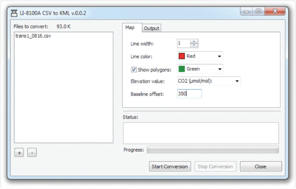
Data exported from the KML converter are displayed as an extruded track, where the Elevation value is used as the variable to plot in Google Earth. The track is shown by a line, the width of which is set with the Line width field, that extends above the ground at a height equal to the Elevation value minus the Baseline offset. Use of a baseline offset allows for small variations in the data to be seen more easily when the data are displayed. Line color sets the color of the track line and the corresponding extrusions from the track to ground level at each data point. The check box next to Show polygons determines whether or not the area between the extrusions is filled, and allows the fill color to be picked. While the track lines are opaque, the polygons are partially transparent.
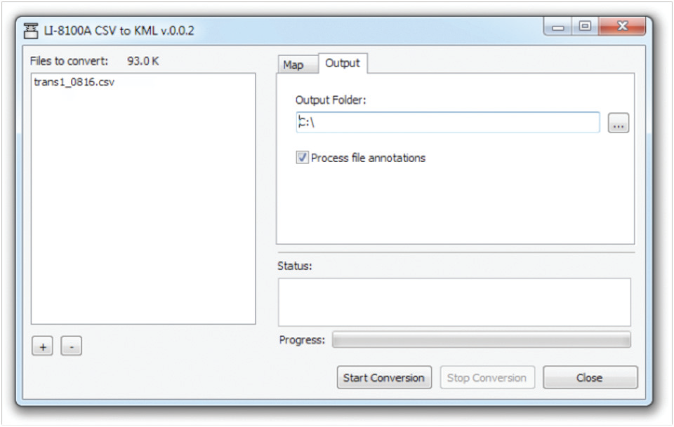
After formatting of the output data has been set up on the Map tab, the Output tab can be used to select where the .kml file will be saved. Select the output directory under the Output Folder, and choose whether or not to process annotations in the data file. Checking the box next to Process file annotations will create a separate .kml file from annotations present in the data, which will display in Google Earth as placemarks. Click Start Conversion to create the .kml file(s).
If Google Earth is installed on the host computer, double clicking the resulting .kml file will launch Google Earth and zoom to the geographic location the file represents. Google Earth’s pan, tilt and zoom tools can then be used to manipulate how the data are displayed.
Considerations for Soil CO2 Flux Mapping
The 8100-405 CO2 Mapping Kit includes a Garmin 18x GPS receiver fitted with Turck connectors for interfacing with the LI-8100A. This receiver uses GPS augmented with WAAS (Wide Area Augmentation System available in North America) to increase accuracy of the position measurement. For the standard GPS measurement, accuracy is better than 15 m, and where WAAS is available typical accuracy is improved to better than 3 m. Accuracy will be degraded where line of sight to satellites is obstructed, objects in the signal path delay signal travel time, or when few satellites are available.
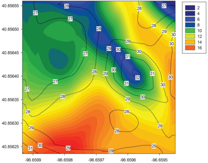
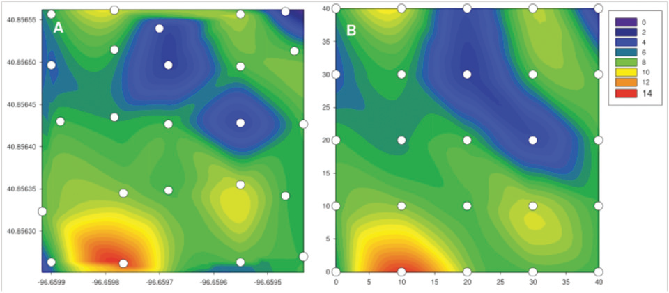
Accuracy of the GPS receiver should be considered when placing soil collars for soil CO2 flux mapping. For measurements made over small areas, placing soil collars closer than the accuracy specification may lead to large errors in flux maps due to the relative size of positional errors to that of the study area. At larger distances between collars small positional errors become less important. Figure 4 shows a comparison between false color plots of soil CO2 flux using latitude and longitude reported by the receiver and using the known relative collar positions. A 10 m collar spacing was used, and it is evident that at this spacing, positional errors have a minor impact on the plot.
To configure the instrument for flux measurements that include spatial data, follow the instructions in the 8100-405 instruction manual. By default all fields reported by the GPS unit will be included in the data file. This can be verified or fields can be removed in the measurement configuration section of the instrument’s interface software.
Exporting Data for Flux Mapping from SoilFluxPro
To get summary records (e.g., soil CO2 flux, curve fit statistics) and spatial data collected in the LI-8100A’s default flux measurement mode into a format that can be plotted or analyzed in your choice of software, data can be exported from SoilFluxPro Software. Data should only be exported after appropriate QA/QC procedures have been performed on the raw records. For more details refer to the SoilFluxPro instruction manual.
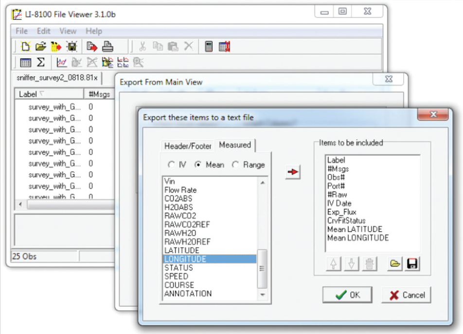
To export the data, open the .81x file using SoilFluxPro and select Export from the File menu or by click the Export icon at the top of the window. This will open the Export from Main View wizard.

Use the radio buttons under Which Observations? to select whether data for all records, or only the selected records will be exported. If no records are selected in the main view then the radio buttons will be grayed out and the wizard will default to all records. Select the Other radio button under Which Columns? and click Define. This will bring up the Export these items to a text file wizard. Click the Measured tab and select the radio button for either the initial value (IV) or the average value (Mean). Scroll through the box on the left hand side of the screen to select LATITUDE and LONGITUDE. Use the red arrow to move these items to the Items to be included list. Any other variable of interest can be added to the list in the same way. When finished choosing variables, click OK, then Export, and select a directory to save the resulting .txt file to.
Notes on Using the GPS Receiver
Mounting: The GPS unit included in the 8100-405 CO2 Mapping kit has a built in magnet to allow the receiver to be easily installed on any magnetic surface (or it can be affixed with tape or hook-and-loop, for example). It can also be affixed using a metric M3 screw and the hole in the base of the receiver. A metal mounting bracket is included in the kit, which supports both mounting options and attaches the GPS unit to the side of the LI-8100A Analyzer Control Unit.
Communication: The GPS unit communicates with the LI-8100A through the instrument’s serial interface. This serial interface is not dedicated to the GPS unit, and serves a dual purpose as one method of connecting the LI-8100A to a computer. When the GPS unit is connected to the LI-8100A, the serial connection cannot be used for communicating with a computer. Instead, wired or wireless Ethernet communication must be used.
An LI-8100A running embedded software version 4.x or above can also communicate wirelessly with a handheld device. However, GPS is only supported in devices running Windows Mobile interface software v1.x or above.