Printable PDF: Capturing and processing soil GHG fluxes using the LI-8100A
Download this content as a pdf that can be saved to your computer or printed.
The LI-8100A Automated Soil CO2 Flux System is designed to measure CO2 efflux from soils using the closed non-steady state transient approach. While CO2 is an important gas in many contexts, it is not the only gas of interest for many research applications. By exploiting some simple hooks in the system a third party analyzer capable of measuring other trace gases can be interfaced with the LI-8100A System and our data processing software (SoilFluxPro) can be used to compute fluxes for these additional gases. In this application note we describe considerations for selecting an appropriate third party analyzer, how to integrate it into the system and the procedure used to compute fluxes of additional gases in SoilFluxPro.
Flow, volume, and pressure considerations
There are three flow loops inside a multiplexed LI-8100A System: the primary sampling loop between the multiplexer and chamber, the subsampling loop between the LI-8100A and the multiplexer, and the pressure regulation loop inside the multiplexer. Each of these loops operates at a different flow rate. The nominal flow rate through the subsampling loop is between 1.5 and 1.7 SLPM at near atmospheric pressure.
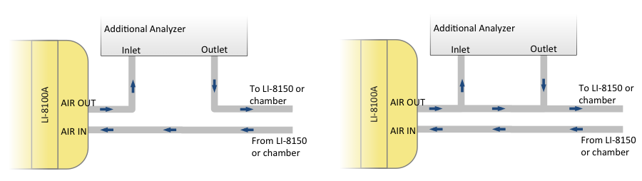
In a multiplexed configuration, the subsampling loop is where any additional analyzer should be placed, either in series with the air outlet from the LI-8100A or in parallel to it (Figure 1). Series placement is possible when the additional analyzer does not use its own internal pump and is capable of operating at the same flow rate and pressure as the LI-8100A. Parallel placement is required when the additional analyzer operates at a different pressure or flow rate lower than the LI-8100A. In either configuration it is possible for the additional analyzer to cause a slight over-pressure on the LI-8100A’s optical bench. Care should be taken to avoid creating flow restrictions in the subsampling loop and where these cannot be avoided it may be necessary to adjust the bias on the pressure regulation loop. To adjust the pressure regulation loop:
- With all plumbing modifications and the additional analyzer in place, note the LI-8100A optical bench pressure when all flow pumps are off.
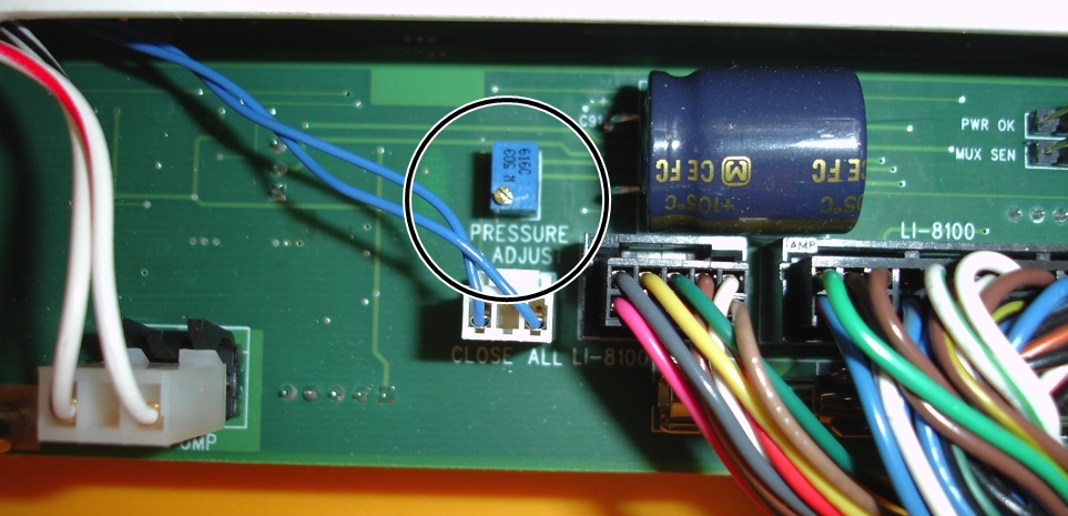
- Open the LI-8150 multiplexer and remove the splash guard that covers the fuses.
- Locate the blue Pressure Adjust potentiometer (up and to the left of the fuses, see Figure 2).
- Turn on all flow pumps and look at the LI-8100A optical bench pressure.
If it is different from the pressure noted in step 1 use a small flat head screwdriver to adjust the Pressure Adjust potentiometer to minimize the pressure difference between when the pumps are on or off. Note that it may not be possible to bring the pressure difference to zero between when the flow pumps are on and off; within ±0.5 kPa would be typical. If there is some offset, the calibration procedures outlined below should be followed to ensure that the LI-8100A performs as expected.
When operating with a single chamber and standalone LI-8100A analyzer control unit, the third party analyzer should be placed on the AIR OUT line from the LI-8100A using one of the plumbing schemes described in Figure 1. The plumbing configuration follows the same guidelines when placing the additional analyzer in the subsampling loop of a multiplexed system. The flow rate between an LI-8100A and a single chamber, and the flow rate in the subsampling loop of a multiplexed system, are both nominally between 1.5 and 1.7 SLPM.
The volume of the additional analyzer will have at least two kinetic effects: 1) it brings additional air to the system, which dilutes trace gas entering the system from the soil surface and reduces the measured trace gas mole fraction rate of change (dC/dt); and 2) it creates a time delay in the onset of a monotonic concentration increase or decrease. Accurate fluxes can still be measured if the added volume is sufficiently small.
The quantitative impact of the added volume on dC/dt can be evaluated by considering the equation used to calculate flux F (mol m-2s-1, equation 1). This equation is derived based on the assumption of a single fixed volume V (m3) with homogeneous air density ρ (mole m-3). For simplicity in this discussion the effects of water corrections are neglected. This however, does not change the conclusions. Thus,

where F is the flux of trace gas (mol m-2s-1), where ρ is air density (mol m-3), dC/dt is the time rate of change in mole fraction of the gas being measured (mol mol-1s-1), and S (m2) is the soil surface area over which the flux occurs. For a flux F, the trace gas mole fraction rate of change dC/dt is proportional to the total number of molecules in the system ρV.
For a well-mixed system, when an additional volume Vadded (m3) that contains a gas of density ρadded is inserted into the system, equation 1 becomes
2

Assuming Vsystem (m3) and Vadded each operate at uniform temperature and pressure, ρsystem = Padded / RTadded and ρadded = Padded / RTadded, where R is the universal gas constant (8.314 Pa m3K-1mol-1), and Tsystem, Psystem and Tadded, Padded are the temperature (K) and pressure (Pa) in the system and additional volume respectively. Substituting these expressions and factoring gives,
3

For data processing using SoilFluxPro, an effective volume Veffective for the addition can be defined for the added analyzer and entered into the software.

Thus, the total volume used in equation 1 becomes simply Vsystem+Veffective and the density is ρsystem. The system density is computed using Psystem from the pressure measurement in the LI-8100A optical bench, and Tsystem from the chamber air temperature. There are inherently small variations in Veffective due to changes in Tsystem and Psystem, but these are generally small and subsequently neglected.
In cases where the volume of the addition operates at a non-uniform temperature and pressure or is not well known, Veffective can be estimated experimentally by plumbing the third-party analyzer in a closed loop and injecting a known volume Vinjection (m3) of pure CO2 into the loop. The gas concentrations in the loop pre-injection C1 (mol mol-1) and post-injection C2 (mol mol-1) are defined as


where NCO2 is the number of moles of CO2 in the additional volume pre-injection, Nadded is the total number of moles in the additional volume pre-injection, and Ninjection is the number of moles of CO2 injected into the loop. Substituting equation 5 into 6 and rearranging to solve for Nadded yields

where  and
and  . Tinjection (K) and Pinjection (Pa) are the temperature and pressure, respectively, of the gas injected into the closed loop. Substituting these into equation 7, and following from equation 4, yields

In practice it is difficult to know Tinjection and Pinjection with great certainty. Making the assumption that Pinjection = Psystem and Tinjection = Tsystem introduces some error in determining Veffective experimentally, but it allows equation 8 to be simplified, eliminating the need to know temperature or pressure.
9

In many cases, the impact of an added volume on flux calculations will be modest as Veffective for many modern trace gas analyzers is small. For example, neglecting the additional volume of an analyzer with an internal volume of 325 cm3, operating at 18.75 kPa and 300.12 K would introduce an error of less than 1.5% for the nominal system volume of a multiplexed system.
By trapping air making its way around the measurement circuit, the volume of a third-party gas analyzer may also introduce an additional time delay and have other effects that can compromise the flux measurement. The magnitudes of these effects are related to the analyzer’s volume Vadded, its operating pressure and temperature, and the flow rate through it. We can qualitatively assess the kinetic consequences of adding the volume by defining a time constant for the effective volume of the added analyzer and comparing it empirically to tested cases. We define a time constant τadded (s)
10

where Uadded is the molar flow rate (moles s-1) delivered to the analyzer, ρadded is air density in the analyzer evaluated at the analyzer’s internal temperature and pressure, and Vadded is its actual volume.
Time constants for different analyzers or model volumes inserted into the LI-8100A subsampling loop are shown in Table 1. We have tested the impact of adding volumes in both series and parallel configurations, and found that accurate fluxes were observed when a volume was added having a time constant of about 7 seconds, but not 17 seconds (Table 1). Based on these results, we expect that third-party analyzers added in series or parallel with time constants less than 5 to 7 seconds may work well. We recommend fluxes made with any other configuration not shown here be validated. Validation can be straightforward if the third-party analyzer measures CO2 as well as other gases of interest.
The configurations reported in Table 1 all affect dC/dt and introduce time delays. But for systems with appropriate time constants, accurate fluxes can be obtained by entering the appropriate volumes, adjusting the dead band to accommodate delays, and computing fluxes using SoilFluxPro.
Calibration considerations
The calibration procedures outlined in the LI-8100A user manual are fine for normal operation of the instrument where optical bench pressure is not significantly altered from ambient. However, when plumbing additional volumes into the system, small pressure differences can cause offsets in the gas measurements when the standard calibration procedure is followed. These offsets tend to be small and may only be apparent when a CO2 measurement is available at two different points in the system.
When operating with a third party analyzer plumbed into the system an alternative calibration routine can be used:
- With the system plumbed for operation with the third party analyzer, turn on the flow pumps and note the optical bench pressure.
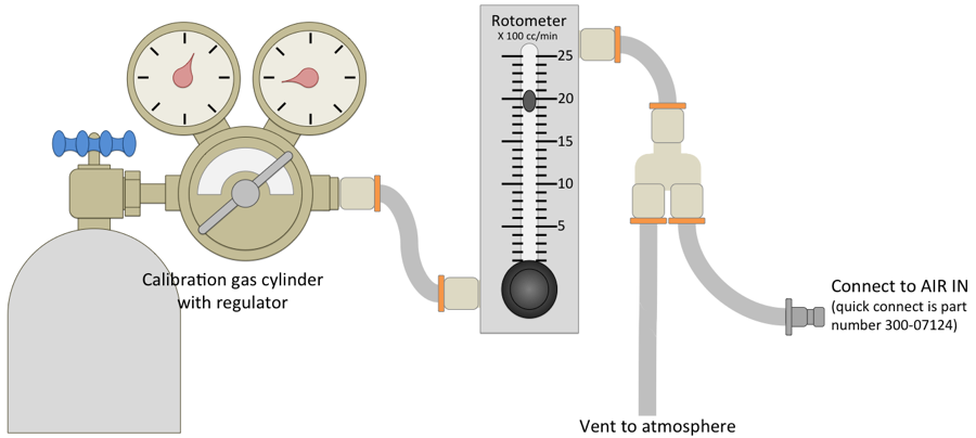
- Disconnect the hose from the air inlet (AIR IN) and connect the calibration rig as described in Figure 3.
- With the flow pumps on, adjust the flow rate through the rotometer such that bench pressure on the LI-8100A is as close as possible to what it was in step 1.
- A slight pressure difference (±0.5 kPa) may be unavoidable and is okay. It is critical however, that flow through the rotometer exceeds the flow through the LI-8100A and that some small excess flow leaves the vent tube in the calibration rig. A flow rate of 2.0 to 2.5 LPM through the rotometer may be suitable to meet the demand of the LI-8100A pump and have a small flow out the vent.
- When the gas concentration reading stabilizes, set the zero, span or span 2 using the LI-8100A interface software as described in the LI-8100A user manual.
- Calibrating the third party analyzer following this same procedure may be wise as well. Check with its manufacturer for calibration details.
Despite careful calibration some offsets may be seen between CO2 and water vapor as measured by the LI-8100A and some third party analyzer plumbed in line with it. These offsets can appear due to a number of reasons, and are not necessarily important in the context of the flux measurement. For water vapor, differences during a given flux measurement may be expected due to interactions with surfaces at different points in the system that lead to a differential time response for water vapor for the two analyzers. For this reason it is important to record both the concentration of the gas of interest and water vapor from the additional analyzer, or where available, record the dry mole fraction for the gas of interest.
For CO2, differences will occur due to an inherent time delay resulting from the additional analyzer being physically separated from the LI-8100A’s analyzer; the magnitude of this delay is related to the volume, flow rate, operating pressure, and location of the additional analyzer. But differences may also occur to due to drift of the LI-8100A over time or pressure induced calibration offsets as discussed previously. It should also be noted that the accuracy of the LI-8100A’s analyzer is specified as 1.5% of reading.
In a closed system where fluxes are computed from a rate of change, measurement of absolute concentration may seem less important than ability of the analyzer to accurately measure a change in concentration. However, because the absorptance measured by the LI-8100A is a non-linear function of CO2 (and water vapor) concentration over its calibration range, the absolute concentration and rate of change are interrelated, and offsets in the absolute concentration may have a small impact on the flux. In practice, this effect is small and arises because the slope of the calibration curve increases with increasing CO2 concentration.
Data integration
Using analog signals
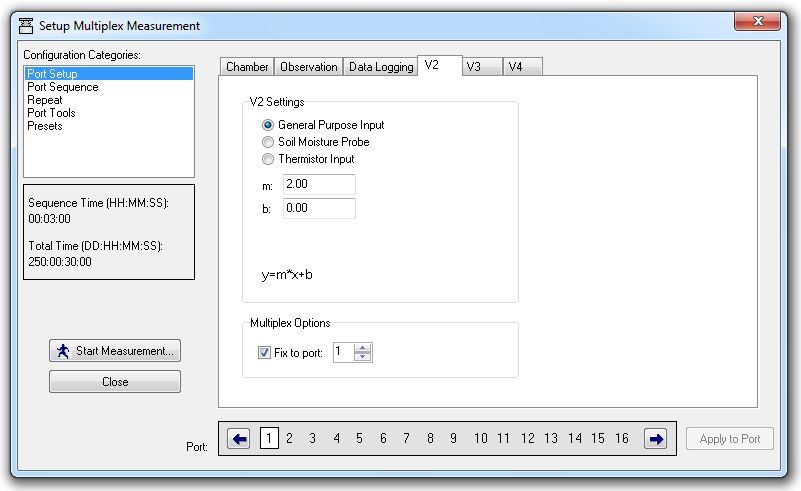
If available on the third party analyzer, its analog outputs can be used to integrate data on the LI-8100A resulting in a single .81x file containing the time series for multiple gas species that can be processed in SoilFluxPro. If the system includes a multiplexer these output channels can be fed into one or more of the three auxiliary inputs available for the 8100-104 or 8100-104C chambers. In software, the auxiliary inputs from a single chamber can be mapped to all ports, allowing the third party analyzer to be connected at only a single location (Figure 4). For single chamber systems, lacking a multiplexer, the outputs must be fed into one or more of the four auxiliary inputs available through the 8100-663 Auxiliary Sensor Interface regardless of the chamber used.
The auxiliary inputs available through either the chambers or the 8100-663 are measured in volts with 13 bit resolution over a 0 to 5V input range. The instrument software supports linear scaling (general purpose input), as well as a Steinhart-Hart conversion (Figure 4).
For integrating data in a multiplexed system an auxiliary input cable (part number 392-08577) is available that connects directly to the auxiliary inputs on the 8100-104 and 8100-104C chambers. This cable provides a weatherized connection at the chamber and bare leads to interface to the third party analyzer’s analog outputs. One cable will be necessary for each channel in use, and due to the cable’s length, the analyzer must be placed near the chamber it is connected to. A 2 m cable (392-07955) is also available that allows the additional analyzer to be attached directly to the LI-8150 in place of a chamber, allowing the LI-8150, LI-8100A and third-party analyzer to be collocated up to 15 m from the chambers. Only one of the 392-07955 cables is required to access all three of the auxiliary inputs. Pin outs for both cables are given in Table 2.
For connecting to the 8100-663 Auxiliary Sensor Interface a user supplied cable with a suitable connection to the third party analyzer on one end and bare leads on the other will be required. For details on how to connect to the auxiliary sensor interface see the LI-8100A user manual.
Using an external data file
Where analog signals are not available, it is possible to integrate a separate data file from a third party analyzer in post processing using the import feature in SoilFluxPro. This allows fluxes to be computed for data collected remotely from the LI-8100A when analog outputs are not available from the additional analyzer. It is necessary that the data to be imported have time stamps that are reasonably synchronized with the LI-8100A; fixed offsets can be accounted for. The import routine will select or generate a data point from the import file for each record of the LI-8100A file. If there is not an exact match, it will pick the two closest values and interpolate. Thus, 1 Hz data is best, but is not required. The import routine supports native text file formats used by a number of gas analyzer manufactures, and can be configured to match a variety of other formats. For details on how to import external files see SoilFluxPro’s user manual.
Time keeping and clock synchronization between the LI-8100A and other system clocks
Importing data from a third party analyzer into the LI-8100A’s .81x files through SoilFluxPro Software is done by matching time stamps between the two data sets. This requires that the two devices keep time relatively consistently between each other. In cases where an offset exists in the timestamps, a fixed offset can be applied and accounted for in SoilFluxPro during importation. This requires, however, that the offset be constant over the entire data set being processed. On short time scales it may be reasonable to assume drift is minimal and that the offset is approximately constant, with any additional small deviations accounted for in the curve fitting process. Over longer time scales, the asynchronous nature of clock drift ensures that without some intervention the offset will not be a constant value.
There is no internal mechanism in the LI-8100A that allows the instrument clock to be synchronized to a standard, or for it to act as a standard for other connected devices. In its typical application, the LI-8100A system runs independently and relies on the user to manually set its clock through its interface software before collecting data.
For users wishing to automate clock synchronization there is hope however. The LI-8100A configuration grammar supports pushing a time and date stamp to the instrument through either its serial or Ethernet interfaces. This allows a computer or microcontroller connected to the instrument to serve as an external standard for the instrument’s clock. In many cases the external standard can be the third-party analyzer (more details below).
Configuration grammar
When a measurement is not active the following command can be used to set the time and date:
<SR><CFG><CLOCK><TIME>{HHMMSS}</TIME><DATE>{YYYYMMDD}</DATE></CLOCK></CFG></SR>
In situations where automated clock synchronization would be desirable, it is unlikely that there will be open windows where a measurement is not active (e.g., continuous sampling with a multiplexed system). Thus, before sending the command to update the clock, it will be necessary to send the following command to end the active measurement:
<SR><CMD><MEAS>STOP</MEAS></CMD></SR>
To restart the measurement, send the following:
<SR><CMD><MEAS>START</MEAS></CMD></SR>
This will restart the measurement using the settings from the active configuration. To avoid file naming errors that will prevent the measurement from restarting, select append mode when configuring and starting the initial measurement through the interface software.
All commands sent to the LI-8100A need to be followed with a line feed (ASCII 10) for the instrument to recognize them. The instrument sends an acknowledgment after receiving a valid command.
8100sync
In cases where the third-party analyzer runs a Windows operating system, clock synchronization can be done using a simple application, 8100sync, and the Windows Task Scheduler.
You can download 8100sync from the technical support website (licor.com/support/home.html) or directly at: https://licor.app.boxenterprise.net/s/7sz6ddmimlskqez39wistcx1qwj56zpx
8100Sync is a tool used to manipulate the clock on an LI-8100A running embedded software 4.0 or above, and includes some basic file management functionality. It is intended to be run from the Windows Task Scheduler at some regular interval to synchronize the LI-8100A clock to PC time. 8100Sync has been tested on Windows Vista, 7 and 10, and may be compatible other versions of Windows.
It consists of two separate executable files: 8100Sync2.0.exe and comscript.exe, and a simple configuration file. 8100Sync2.0.exe provides a graphical interface for comscript.exe with real-time status updates and an editor for the configuration file. Comscript.exe handles communication with the LI-8100A and can be run independent of 8100Sync2.0.exe. When run independently comscript.exe provides no user feedback, but will trigger a save-only version of the configuration editor if problems are found with the configuration file. 8100Sync2.0.exe is dependent on comscript.exe and the application will automatically exit when comscript.exe is done executing; this allows either application to be used in the Task Scheduler. When the configuration editor is opened from either application, comscript.exe stops and will restart when the editor is closed.
Full details on how to use 8100Sync and how to configure the Task Scheduler can be found in the documentation included with the application.
Curve fitting and computing fluxes using SoilFluxPro
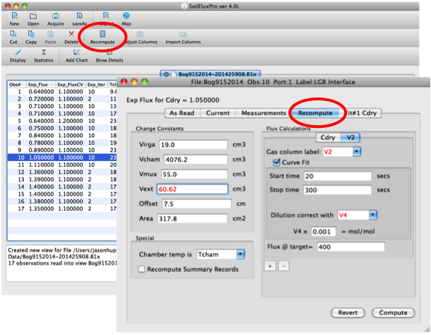
To compute fluxes for additional variables included in the .81x file access the recompute dialog; This can be done for all records in a file using the Recompute icon at the top of the SoilFluxPro window, or for a single record by double clicking the record in the summary view and going to the Recompute tab in that record’s observation view. Figure 5 shows the recompute window for a single record.
In the recompute dialog, click the + under Flux Computations to add an additional variable for which fluxes are to be computed. Under Gas column label: select the variable. In the example here methane mole fraction was logged as umol/mol through auxiliary input V2. Check the box for Curve Fit and select start and stop times for the curve fit. These may need to be adjusted later. Under Dilution correct with select the channel where water vapor was recorded from the additional analyzer and use the scalar below it to scale the value to mol/mol. In the example, water vapor was logged on V4 as mmol/mol, so it needs to be multiplied by 0.001 to convert to mol/mol. If the third party analyzer reports dry mole fraction, then no additional dilution correction is needed. Under Vext input the effective volume determined following the guidelines presented under Flow, volume, and pressure considerations. In this case the additional analyzer has an actual volume of approximately 325 cm3 and operates at 18.75 kPa and 300.12 K. At a chamber pressure of 100 kPa and temperature of 298.5 K the effective volume was 60.62 cm3.
It should be noted that in the example presented here effective volume is treated as a constant. But in practice chamber temperature and pressure are typically not constant, leading to an effective volume that may be different for each measurement. However, when the effective volume is small relative to the total system volume, the error associated with treating it as a constant may not be important. For the example presented here, changing the chamber temperature by 25 °C affects the total volume by less than 0.1% and for a 5 kPa change in chamber pressure, the effect is less than 0.04%.
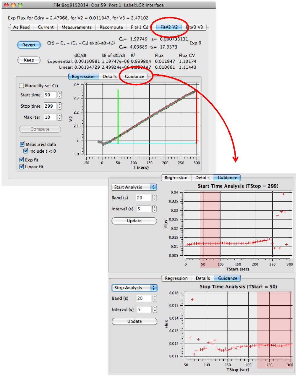
Open the observation view for a record and go to the tab for the additional flux computation. In the example shown here, the tab is labeled Fit#2 V2 (Figure 6). Use the Guidance tab to determine appropriate start and stop times for the curve fitting. In the example dataset, a start time between 40 and 100 seconds and a stop time of greater than 220 seconds would work (shaded areas in Figure 6). For the start time look for the initial plateau and select a time in that window. For stop time, select a time after the values level off. If the Stop Time Analysis curve does not level off or is very noisy, it is possible that the measurement length was too short. Once appropriate start and stop times have been determined it will be necessary to go back and recompute the data set if these times differ from the times used in the initial flux computation.
Note that for gas species with large fluxes and low resistance to diffusion in the soil, long measurement periods may lead to underestimations of the final flux due to buildup of the gas in the soil air space during the measurement. For gas species with low fluxes, such as methane, long measurement periods may be required to get enough data for a good curve fit. This means when measuring methane and carbon dioxide together, it will often be necessary to use different stop times for the two gases in the flux computation, with the stop time for carbon dioxide occurring much before that of methane.
Once satisfied with the curve fitting and summary values, the Export icon at the top of the main SoilFluxPro window can be used to export the summary values. For additional details on computing additional fluxes and exporting data see the SoilFluxPro manual accessed under Help in the software.
Example 1: Measurements using the Los Gatos Research Ultra-Portable Greenhouse Gas Analyzer
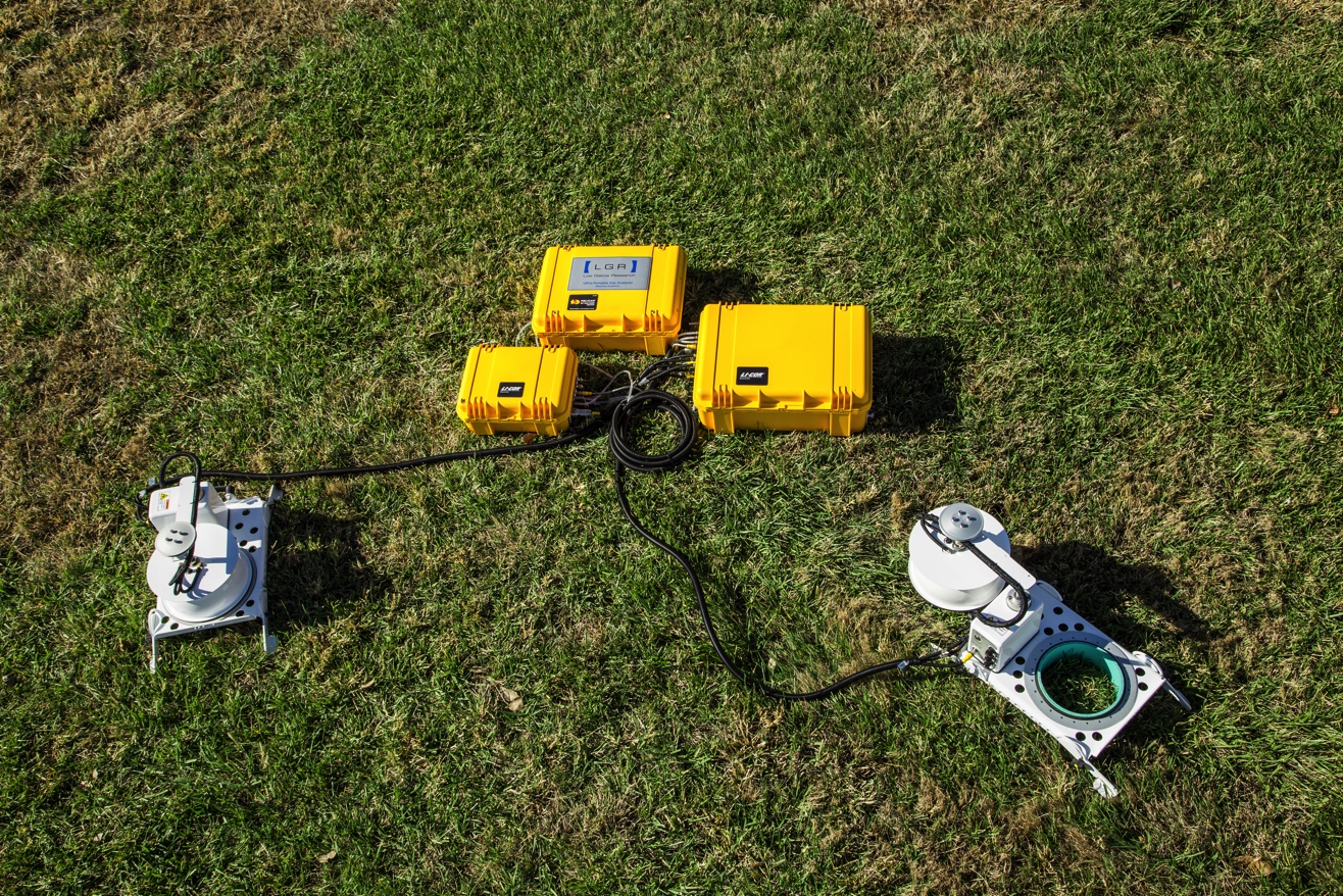
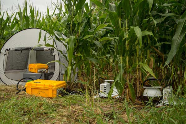
An Ultra-Portable GGA (model 915-0011) from Los Gatos Research, a member of the ABB group, was integrated into a multiplexed LI-8100A System (Figure 7) using a parallel plumbing configuration. Data from the analyzer was brought into the LI-8100A System using its analog outputs. Data collection was tested using both connection schemes described under Data Integration. Wiring for the two cable sets tested is described in Table 3.
The Ultra-Portable GGA had an actual volume of approximately 325 cm3 and operated at 18.75 kPa and 300.12 K. Flow rate through the Ultra-Portable GGA was 0.8 SLPM. A chamber pressure of 100 kPa and temperature of 298.5 K was used to compute the effective volume for the Ultra-Portable GGA and an effective volume of 60.62 cm3 was used for all flux computations.
Initial experiments were done in the lab to compare a known flux to the flux as determined from each analyzer’s time series data. Known fluxes were generated by injecting pure CO2 at a constant rate through a mass-flow controller into a sealed collar below an 8100-104 chamber. Data from these experiments are presented in Table 4 and show that for an artificial flux produced by mass-flow the LI-8100A and Ultra-Portable GGA give the same and expected result.
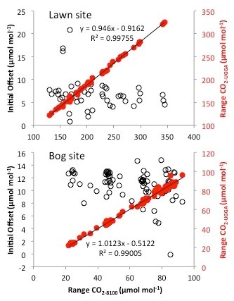
The system was deployed on a mowed lawn and an artificial peat bog in Lincoln, NE to measure fluxes of carbon dioxide and methane. The two analyzers were cross calibrated prior to the laboratory experiments, but no subsequent calibration was performed prior to the field deployments. Figure 8 shows a comparison of the ranges and initial offsets in carbon dioxide concentration as reported by the two analyzers. While they showed a rather variable offset in concentration at the start of each measurement, the magnitude of change in concentration over each flux measurement was very similar for both analyzers at both sites.
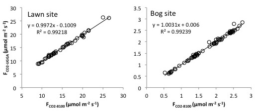
Comparisons were made between the diffusive fluxes of carbon dioxide computed from these data and are presented in Figure 9. Fluxes at the lawn site were quite large during the deployment due to warm weather (mean temperature of 25.7 °C) and abundant soil moisture, and quite low at the artificial bog, presumably due to cooler temperatures (mean temperature of 19.4 °C) and low gas conductance of the saturated peat. Once fit with appropriate start and stop times for the curve fits, the carbon dioxide fluxes from both analyzers at both sites showed little difference (approximate difference of 0.3%) despite the offsets observed in the absolute concentrations as reported by the two instruments.
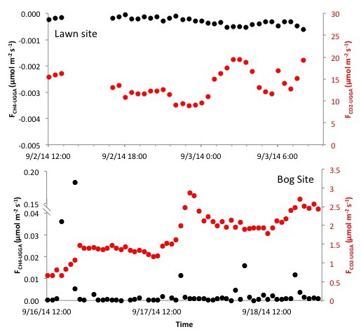
Methane fluxes at the two sites were small, but consistent with expected trends given soil conditions (Figure 10). At the lawn site a small negative flux was observed (mean of -3.3x10⁻⁴ μmol m-2 s-1), presumably due to methane oxidation. At the artificial bog fluxes were nominally zero for most measurements, but did show positive fluxes (maximum of 0.18 μmol m-2 s-1) in the late afternoon when the soil under the chamber was exposed to direct solar radiation.
Example 2: Measurements using the Picarro G2508 analyzer
A five-species gas analyzer (model G2508) from Picarro, Inc. was integrated into a multiplexed LI-8100A System (Figure 11) using a parallel plumbing configuration. Data from the G2508 were logged to the analyzer’s hard disk and merged with the LI-8100A’s data in post processing using SoilFluxPro’s import utility. 8100Sync was run on the G2508 from the Windows Task Scheduler, and used to synchronize the LI-8100A’s clock to the clock of the G2508 every day at midnight. Clock synchronization was done over Ethernet using a direct connection between the LAN ports on the two instruments.
Flow through the G2508 was provided by the analyzer's vacuum pump and additional external plumbing was required to connect the two devices. While the G2508 optical bench has a specified volume of approximately 35 cm3, the additional external plumbing and pump represented a significant fraction of the total additional volume the analyzer added to the system. This complicated the computation of Veffective as temperature and pressure were not uniform through the total volume and were only known in the optical bench. As such, Veffective was determined for the G2508 experimentally as described in Flow, volume, and pressure considerations. Results are presented in Table 5.
The system was deployed on a mowed lawn and an artificial peat bog in Lincoln, NE to measure fluxes of carbon dioxide and methane. During deployment at the lawn site the two analyzers were cross calibrated by passing dry standard gases through them to ensure they were functioning correctly.
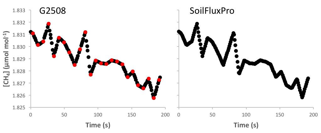
At both sites methane fluxes were relatively small and consistent with expectations based on soil conditions (Figure 12). At the lawn site predominately small negative fluxes were observed (mean of -1.8x10⁻⁴ μmol m-2 s-1) and were attributed to methane oxidation in the soil. Accumulation curves for methane at this site showed an oscillation in concentration across the curve (Figure 13). While similar oscillations have been observed in accumulation curves due to pressure perturbations or poor mixing in the chamber, in this case the oscillations appear to be due to the asynchronous nature of the G2508’s measurements and concentration changes approaching the instrument’s limit of precision (<10 ppb + 0.05% of reading, precision for raw signal). Methane was measured approximately every eight seconds by the G2508 and was up-sampled by the instrument to generate an approximately one sample per second times series. At the bog site, where fluxes were higher (mean of 1.2x10⁻² μmol m-2 s-1) and larger changes in methane concentration were observed, similar oscillations were not evident in the accumulation curves.
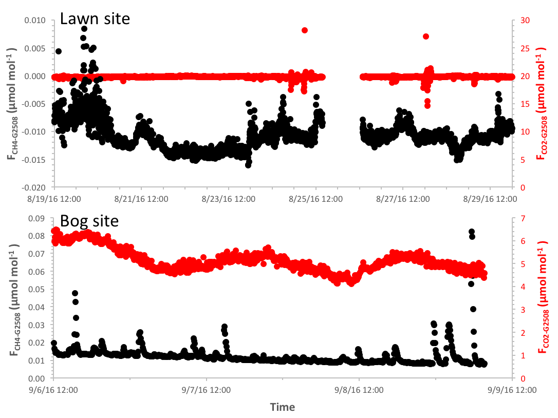
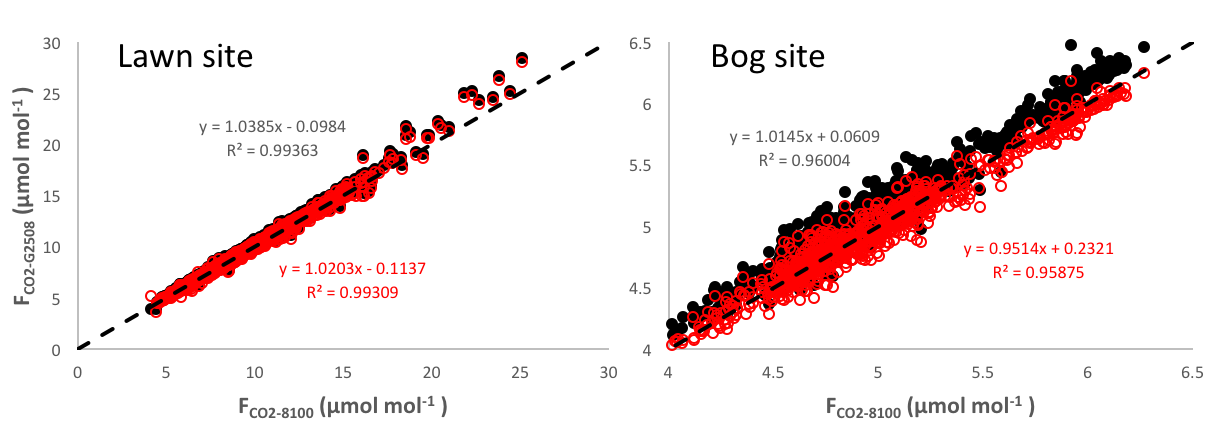
At both sites carbon dioxide fluxes were of a relatively similar magnitude; mean of 8.8 μmol m-2 s-1 at the lawn site and 5.0 μmol m-2 s-1 at the bog site as measured by the LI-8100A. A cross comparison was made between the flux of carbon dioxide computed from the LI-8100A’s data and that of the G2508 (Figure 14). After careful optimization of the measurement start times, a small residual difference was observed in the fluxes computed from carbon dioxide dry mixing ratio, with fluxes computed from the G2508’s data on average 2.7% larger than those computed from the LI-8100A. This offset was consistent across data from both deployments and did not appear to be due to a calibration offset between the two instruments, as they reported expected values when sampling dry standard gases during the initial cross calibration. Fluxes computed using a traditional dilution correction applied to the G2508’s wet mole fraction data to get dry mixing ratio (Hupp 2011), were more similar to the LI-8100A fluxes (mean difference of 0.27% across both sites). The dilution correction used to compute dry mixing ratios on board the G2508 includes an additional spectroscopic correction not included in a traditional dilution correction (Rella 2010).
Example 3: Recommended integration procedures for Aerodyne, Inc. Dual-TILDAS analyzers
A Dual-TILDAS analyzer from Aerodyne, Inc. fitted with a Super Cell optical cell (2.7 L internal volume), was tested with a multiplexed LI-8100A system. While the tested analyzer, pump and optical cell configuration proved to have a time constant too long for use with the LI-8100A system. The tests provide insight and a basis for recommended integration schemes for other Dual-TILDAS instruments that should work well with the LI-8100A system.
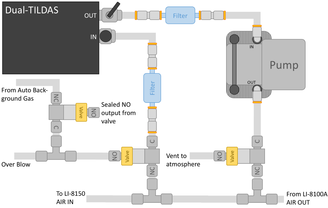
The recommended plumbing configuration for a Dual-TILDAS analyzer connected to the LI-8100A system is shown in Figure 15 and follows the configuration used in our internal testing. The analyzer should be plumbed in parallel to the AIR OUT line from the LI-8100A as shown using the 9981-189 hose assembly, or similar user provided plumbing assembly. Flow through the analyzer needs to be provided by an independent pump cable of drawing sufficient vacuum on the analyzer’s optical cell. In testing we used a Pfiffer MVP 015-4 PK T05 064 connected to the analyzer’s outlet. This pump provided a flow rate of approximately 1.0 SLPM at the analyzers inlet, with an optical cell pressure maintained at 6.7 kPa. Cell pressure and flow should be set using inlet and outlet valves following the standard recommendations of Aerodyne Inc. Filters (recommended filter: United Filtration Systems Inc. DIF-BN60) should be included on both the analyzer’s inlet and outlet to protect the optical cell from contamination and a series of solenoid valves (recommended valve: Parker 009-0294-900) may be included in the subsample loop to allow an auto-background gas to be provided to the Dual-TILDAS under its own control.
It is recommended that time series data for flux measurements be logged separately on the LI-8100A and Dual-TILDAS and fluxes computed in post processing by merging the data files in SoilFluxPro. Time synchronization between the two instruments can be done over Ethernet or serial using 8100Sync configured to run in the Windows Task Scheduler onboard the Dual-TILDAS.
During testing, Veffective and time constants were derived for the test setup following the procedures outlined in Flow, volume, and pressure considerations. Veffective, as determined from injections of pure CO2, was 267.2 cm3 and that, computed using the analyzer’s internal volume, was 178.2 cm3; the difference between the two presumably owing to the volume of the components in the analyzer’s subsampling loop.
The time constant for the analyzer as computed from the measured flow rate in its subsample loop and its measured Veffective was 16.3 seconds. In previous work, we have observed that time constants around this value had too large of impact on system kinetics for a closed transient measurement.
While the pump used in testing provided too low a flow rate to be useful with an analyzer fit with the Super Cell, it could be expected to work with a Dual-TILDAS fit with the standard optical cell (0.67 L internal volume). Assuming the same subsample loop contribution to Veffective and the same operating pressure, at 1.0 SLPM the expected time constant for the standard cell would be approximately 8 seconds. To work with the Super cell, a flow rate of greater than 2 SLPM would be needed at the tested operating pressure (6.7 kPa) and temperature (24 °C).
While its flow rate is expected to be suitable for use with the standard optical cell, the tested pump may not be suitable depending on the gas species desired for measurements. The tested pump uses the fluoroelastomer FPM for its internal seals and diaphragms, which may interact with certain gas species. When new, the pump off-gassed all species measured by the analyzer during testing (CO, CH4, CO2, N2O, C2H6) and had to be purged with air for several hours before it could be used for measurements. After purging the pump, no impact was observed during testing due to the FPM materials inside the pump.
For recommended pumps operating at higher flow rates and/or different internal materials contact Aerodyne Inc.
References
Hupp, J.R. 2011. The Importance of Water Vapor Measurements and Corrections. LI-COR, Inc., Application Note 129.
Rella, C.W. 2010. Accurate Greenhouse Gas Measurements in Humid Gas Streams Using the Picarro G1301 Carbon Dioxide/Methane/Water Vapor Gas Analyzer. Piccaro, Inc., White Paper.
Useful Part Numbers
| Part Number | Description |
|---|---|
| 8150-250 | Bev-a-line tubing (15m roll) |
| 300-07385 | ¼” Quick-connect “T” fitting |
| 300-03367 | ¼” Quick-connect “Y” fitting |
| 300-03123 | ¼” Quick-connect straight union |
| 300-07124 | Male stainless steel quick-connect (connects to LI-8100A AIR IN) |
| 300-07125 | Female stainless steel quick-connect (connects to LI-8100A AIR OUT) |
| 300-15313 | Swagelok straight fitting (connects 9981-189 to Picarro G2805) |
| 294-03334 | 0-2.5 LPM flow meter (rotometer) |
| 300-08118 | 1/8” NPT to ¼” Quick-connect right angle fitting (two used with rotometer) |
| 392-08577 | Auxiliary sensor input cable for 8100-104 or 8100-104C chambers |
| 392-07955 | Turck to bare leads cable, 2 m long |
| 314-03430 | Male DB-9 connector with shielded housing (used to access Ultra-Portable GGA’s analog outputs) |
| 9981-188 | Pre-assembled Turck to DB-9 cable for connecting the Ultra-Portable GGA to the LI-8150. |
| 9981-189 | Pre-assembled hose assembly for plumbing additional analyzers in parallel to the LI-8100A subsampling loop. |