Equation Summary

The LI-830 and LI-850 compute CO₂ concentrations using an equation of the form

A‑1

where c is concentration, f() is the calibration function, a" is the absorptance, g (a,P) is the pressure correction, S(a) is the span, and T is the temperature (°C) of the gas in the cell, typically 51.5 °C. Absorptance is computed from

A‑2

a' is a span corrected absorptance, and g(a,P) is the pressure correction.

A‑3

S(a) is the span function, and raw absorptance a is computed from

A‑4

where V and V_o are the raw detector sample and reference readings, and Z is the zeroing parameter.

Span is a linear function of absorptance.

A‑5

H₂O Equations (LI-850 only)

Absorptance a_w for water vapor is computed from

A‑6

where V_w and V_wo are the sample and reference raw detector readings, and Z_w is the zero parameter. The pressure correction for water vapor is an empirical function g_w() of absorptance and pressure P:

A‑7

The value of P_o is 99 kPa. When the pressure correction is not enabled, g_w() is simply 1.0. Water vapor concentration W (mmol mol^-1) is computed from

A‑8

where f_w(x) is a third order polynomial whose coefficients are given on the calibration sheet.

A‑9

CO₂ Equations

The measurement of CO₂ is a bit more complicated than for H₂O because of the influence of water vapor. There is a slight direct cross sensitivity in the CO₂ signal to H₂O. This is measured at the factory and accounted for in the computation of absorptance (equation A‑10). There is also a band broadening effect that is accounted for in the computation of concentration (equation A‑14).

CO₂ absorptance ac is computed from

A‑10

where V_c and V_co are the raw detector signals for sample and reference, Z_c is the CO₂ zero parameter, and X_wc is a cross sensitivity parameter for the effect of water vapor on CO₂. Its value is reported on the calibration sheet as XS=.

The empirical pressure correction function g_c() depends on CO₂ absorptance and pressure:

When P = P_o, g_c() = 1.

When P < P_o

A‑11

where a = 1.10158, b = -6.1217E-3, c = -0.266278, d = 3.69895, and z is the asymptotic value of absorptance, obtained from the calibration coefficients (equation A‑15).

A‑12

When P > P_o

A‑13

where X, A, and B are computed as in equation A‑11. CO₂ concentration C (µmol mol^-1) is computed from

A‑14

where f_c(x) is a function whose inverse is a double rectangular hyperbola, and whose coefficients (a1…a4) are given on the calibration sheet.

A‑15

Solving equation A‑15 for C yields the calibration function

A‑16

Where

A‑17

ψ(W) accounts for band broadening by water vapor.

A‑18

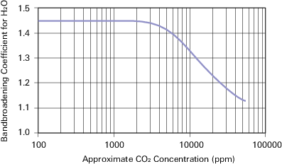
The band broadening coefficient h(a_c) has been determined to be 1.45 for the instrument for CO₂ concentrations near ambient. At higher concentrations, the value decreases. We capture this behavior with an empirical relationship (equation A‑19).

A‑19

Where z is from equation A‑12, and b_w is the low concentration band broadening coefficient: 1.45. This is the value shown on the calibration sheet as BB = 1.45. The typical relationship between h(a_c) and CO₂ concentration is shown in Figure A‑1. (‘Typical’ because the exact relationship depends on the relationship between absorptance and CO₂, which is the calibration curve.)

Note: We formulated equation A‑19 with 0.64b_w – 0.64 instead of the simple equivalent (0.29) because this allows band broadening corrections to be turned off by setting b_w to 1. When b_w =1, h(a_c) = 1 everywhere. Also, to avoid computational problems (underflows, overflows, and division by zero) we constrain the argument a_c when computing h(a_c) to be 0.1 < a_c ≤ z. a_c - 0.1 is typically equivalent to about 600 ppm.

Calibration Equations

The following equations describe the implementation of zero and span calibrations.

Zeroing H₂O (LI-850 only)

When the command for zeroing water is received, the LI-850 computes the water zero from equation A‑20, where and are averaged for 5 seconds.

A‑20

Zeroing CO₂

When the command for zeroing CO₂ is received, the instrument computes the CO₂ zero term from equation A‑21, where , , , and are averaged for 5 seconds.

A‑21

Spanning H₂O (LI-850 only)

When the command for setting the span for H₂O is received, along with the target concentration W_T, from the target concentration, the target absoprtance a_T is computed from

A‑22

LI-850 computes S_w0 from equation A‑23 , where is averaged over five seconds.

A‑23

where

A‑24

The instrument retains the following values, which are used for subsequent secondary spans:

A‑25

Secondary Span H₂O (LI-850 only)

When the secondary span command for H₂O is received, the instrument computes new values for both S_w0 and S_w1. First, it measures a new and computes a new from equation A‑24. Then, it uses these plus the retained values ( and from the previous normal span) to compute

A‑26

Given the new span slope S_w1, it updates the span offset S_w0 by equation A‑23.

Spanning CO₂

When the command for setting the CO₂ span is received, along with the target concentration C_T, the instrument computes S_c0 from equation A‑28, where and are averaged for 5 seconds.

A‑27

A‑28

where

A‑29

Note that

A‑30

We need acT to compute , but acT depends on . We resolve this by using an approximation (equation A‑31) instead when computing equation A‑30

A‑31

The instrument retains the following values, which are used for subsequent secondary spans, if necessary:

A‑32

A‑33

Secondary Span CO₂

When the secondary span command for CO₂ is received, the instrument computes new values for both S_c0 and S_c1. First, it measures a new and computes a new β_c from equation A‑29. Then it uses these, plus the retained values (a_c1 and β_c1 from the previous normal span) to compute

A‑34

Given the new span slope S_c1, it updates the span offset S_c0 by equation A‑28.