Soil gas flux measurement theory

Gases in soil are produced by a variety of biological mechanisms, including root respiration, decay of organic matter, and microbial activity. Rainwater can have direct effects as well by displacing gas in soil pore spaces and by interacting with limestone soils. Thus, soil gas fluxes are dependent on soil temperature, organic content, moisture content, precipitation, and have a great deal of spatial variability.

Soil gas fluxes are also extremely sensitive to pressure fluctuations. An unvented chamber will induce significant pressure increases just by being placed onto a soil collar or measurement area. Soil water evaporation and heating of the air in the chamber head space also induce pressure increases in an unvented chamber. Therefore, the Smart Chamber is vented so that pressures inside and outside the chamber are in a dynamic equilibrium.

The chamber is designed to mitigate factors that can induce variation in measurements with the following features:

• A bellows-controlled closure mechanism that ensures that placement of the chamber has the same negligible effect with each measurement sample.
• A patented chamber vent that maintains ambient pressure inside the chamber, even in windy conditions.
• Soil collars, which, after installation, ensure consistency between samples.

Gases move from the sites of production to the atmosphere primarily by diffusion through air-filled pores and cracks in the soil, but movement can also be driven by local changes in pressure due to wind, or by volumetric displacement from rain. The air-filled porosity of the soil varies with soil type and moisture content, so these characteristics can have significant effect on the movement of gas through soils.

The Smart Chamber uses the rate of increase of trace gases in the measurement chamber to estimate the rate at which gases diffuse into free air outside the chamber. For such an estimate to be valid, conditions must be similar inside and outside the chamber. These conditions include the concentration gradient driving diffusion, barometric pressure, temperature, and moisture of the soil.

Because there is an increase in mole fraction of the gas being measured inside the chamber, the gradient of gas diffusion between the soil surface layer and air are not exactly the same inside and outside the chamber. The diffusion rate is estimated and corrected for using an analytical technique that takes into account the effects of increasing chamber gas concentration on the diffusion gradient. This makes it possible to estimate the initial rate of gas increase that occurred immediately after the chamber closed.

It is also important to consider the effect of the presence of the chamber on gas gradients within the soil. Detailed diffusion model studies have shown that chambers can alter gas concentration gradients in the soil, leading to errors in flux estimates. For CO₂ and methane, it is generally recommended that measurements be limited to 90 to 180 seconds in order to keep gas concentration changes as small as possible to minimize this effect. Some gases such as H₂O may require longer measurements, up to 15 minutes or longer, to reliably calculate fluxes.

Soil gas flux varies substantially in both space and time. The Smart Chamber can be used to sample both types of variability. The survey-chamber style design of the Smart Chamber allows for rapid measurements to be made at many sites, but can also be used to make longer-term measurements for specific applications or experiment types with or without multiple repetitions at a single site.

The survey measurement cycle

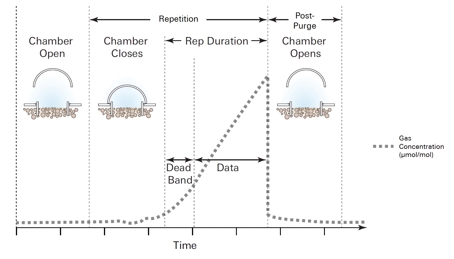
When the Smart Chamber is placed on a soil collar, it will remain open until the measurement is started. When the measurement is started, the bellows pump closes the chamber. Upon closing, the instrument begins logging data, and the dead band starts. The instrument continues to record data for the length of the repetition, and then the chamber opens and pauses for the extra duration. At this point, the measurement cycle is repeated for the specified number of repetitions or the Smart Chamber is removed from the soil collar and taken to a different collar for a new measurement.

Terminology

A repetition represents a single survey measurement and includes the period of time from when the chamber starts closing, the dead band, and the actual measurement logging. A measurement may consist of multiple repetitions at a single collar. Once the desired number of repetitions is completed and the chamber opens after the final repetition, the Smart Chamber can be removed from the soil collar and transported to the next soil collar.

The dead band is the time period that starts when the chamber closes completely, and continues until steady mixing is established and the measurement begins. The dead band requirement changes depending upon the chamber geometry, system flow rate, collar, and site characteristics. A dead band between 10 and 30 seconds generally provides adequate mixing, but the actual time can (and should) be optimized in post processing in SoilFluxPro™ Software.

Lastly, the post-purge is the amount of time during which the pump continues to run and air flows through the chamber as it begins to open, after the measurement is complete. This is important in certain cases where environmental factors may influence the amount of gas or moisture that is present in the sampling lines. For example, in hot, moist conditions, you may want to increase the post-purge to ensure that the gas sampling lines are purged of moisture that may condense in the lines, before the next measurement using that chamber is started. In most cases, a post-purge of about 45 seconds is adequate.

Deriving the flux equation for CO₂

The Smart Chamber can be used to measure fluxes of many trace gases that can be reliably detected with compatible gas analyzers. The flux equation remains the same for all gases. However, CO₂ provides an ideal model for demonstrating the derivation of the flux equation, which is presented here.

At constant pressure, the total rate at which water evaporates into the chamber sf_w (mol s^-1) is balanced by a small flow rate of air out of the chamber u (mol s^-1). The CO₂ mole fraction of the air outside the chamber is c_a, inside the chamber is c_c, and in the soil is c_s, all in mol mol^-1. The chamber air water vapor mole fraction is w_c (mol mol^-1). The rate constant k (s^-1) characterizes leaks (if any) due to diffusion of CO₂ between the soil chamber and outside air. The chamber volume v includes the volume of the pump and measurement loop.

A chamber of volume v (m³) and surface area s (m²) sitting over the soil, which has CO₂ efflux rate f_c (mol m^‑2 s^‑1) and water evaporation flux rate f_w (mol m^‑2 s^‑1).

The mass balance equations for CO₂, water vapor, and air take the form

C‑1storage = flux in - flux out

We neglect the effects of leaks for now, but we will consider them later.

CO₂ mass balance

C‑2

H₂O mass balance

C‑3

Air mass balance

C‑4

is the number density of CO₂ in the chamber, is the number density of water vapor in the chamber, and is the total number density of air in the chamber (all in mol m^-3); , where is the number density of dry air in the chamber.

The number density of air is given by the ideal gas law, , where R is the gas constant (8.314 Pa m³ K^-1 mol^-1), and T_K is the absolute temperature (K). From equation C‑4, with ρ and T_K constant, and sf_w >> sf_c,

C‑5

Combining equations C‑3 and C‑5, and noting that , we find

C‑6

Combining equations C‑2, C‑5 and C‑6 gives

C‑7

Equation C‑7 can be simplified by defining , which is the chamber CO₂ dry mixing ratio, corrected for water vapor dilution, reported in units of µmol/mol. This is different from C_dry, the CO₂ dry mole fraction, reported in units of parts-per-million (ppm) in the data output.

Differentiating we find,

C‑8

Substituting this into equation C‑7 gives

C‑9

Equation C‑9 has an important advantage over equation C‑7 because it is not necessary to estimate the rate of increase in water vapor mole fraction. In most measurements, the water vapor mole fraction increases in a highly non-linear fashion, and the rate is estimated with a linear function. Thus, in effect, equation C‑7 forces us to use average values for and . But with equation C‑9, the dilution correction is made point-by-point, and estimates of the initial values at time zero are used to estimate f_c at the instant the chamber closed. This is both easier and more accurate than the procedure required to implement equation C‑7.

In order to use equation C‑9 the initial values must be known for ρ and T_K (to compute ρ_c), as well as the initial values for w_c and . After the chamber closes, the Smart Chamber performs a linear regression with time on the first 10 values of each measured variable. The initial values of ρ, T_K and w_c are obtained from the time zero intercepts of these regressions; however, finding the initial value for requires a little more work.

To do this, f_c is defined in terms of the CO₂ mole fraction gradient across the soil- to-chamber interface and a transfer coefficient, to obtain

C‑10

where c_s is the CO₂ mole fraction in the soil surface layer communicating with the chamber (mol mol^-1), g is conductance to CO₂ (m s^-1), and ρ_c is the density of air (mol m^-3). The soil and chamber must be isothermal for equation C‑10 to hold.

Combining equation C‑10 with equation C‑9, considering all variables except c_c' to be constant, and rearranging, gives

C‑11

where . When w_c = w_s, c_s', gives the water vapor dilution-corrected CO₂ mole fraction in the soil layer communicating with the chamber. We do not expect w_c to equal w_s exactly, but most of the time they will differ by less than 0.02 mol mol^-1 or so, which introduces only a small uncertainty in c_s'. If c_s' is taken as a constant, then equation C‑11 can be integrated to give

C‑12

where α = sg v^-1 is a rate constant (s^-1) and c_c'(0) is the initial value of the dilution- corrected CO₂ mole fraction when the chamber closes. The rate of change in c_c'(t) at any time can be computed from the derivative of equation C‑12.

C‑13

Calculating the flux from measured data

In the Smart Chamber, equations C‑9, C‑11 and C‑12 are implemented in a form that presents the variables in more familiar and intuitive units. Equation C‑9 is computed as

C‑14

where F_c is the soil CO₂ efflux rate (μmol m^-2 s^-1), V is volume (cm³), P₀ is the initial pressure (kPa), W₀ is the initial water vapor mole fraction (mmol mol^-1), S is soil surface area (cm²), T₀ is initial air temperature (°C), and is the initial rate of change in water vapor dilution corrected CO₂ mole fraction (μmol mol^-1 s^-1).

Examine Figure C‑1 to see C'(t) vs t data that were obtained from a soil CO₂ flux measurement with two observations. The data are marked to show when the chamber closed and when it opened.

The dead band is the time until steady chamber mixing is established, and typically lasts 10s to 30s. After mixing is stable, the data are fit with an empirical equation that has a form similar to equation C‑12:

C‑15

where C'(t) is the instantaneous water-corrected chamber CO₂ mole fraction, C₀' is the value of C'(t) when the chamber closed, and C_x' is a parameter that defines the asymptote, all in μmol CO₂ per mol dry air (µmol mol^-1); a is a parameter that defines the curvature of the fit (s^-1).

The initial value of C'(t), called C₀' in equation C‑15, is computed from the intercept of a linear regression of the first 10 points after the chamber closes. This is used as a parameter in the non-linear regression that fits equation C‑9 to the C'(t) vs t data between the end of the Dead Band and the end of the observation. This regression yields values for the parameters C_x', a and t₀. t = t₀ represents the time when C'(t) in equation C‑15 equals its initial value when the chamber closes, or C'(t₀) = C₀'. The delay between the instant the chamber closed and t₀ gives the time required to establish steady mixing. CO₂ offsets or time delays can occur when the chamber closes, and these events can cause t₀ to be positive or negative in value.

All the initial values needed to obtain the soil CO₂ efflux rate, F_c, in equation C‑9 can now be computed. The initial values P₀, T₀ and W₀ are all obtained from the intercepts of linear regressions of the first 10 measurements of P, T and W after the chamber closes. The rate of change of dilution-corrected chamber CO₂ mole fraction can be computed at any time from

C‑16

When t = t₀,

C‑17

Equation C‑17 gives an estimate of the rate of change in C' at the instant the chamber closed. This value must be estimated mathematically. It cannot be measured directly at any time during the measurement because imperfect mixing prevents an accurate estimate early in the measurement cycle, and later in the cycle, the increasing chamber CO₂ concentration continuously reduces the gradient between soil and chamber. This suppresses the rate, as can be seen from equation C‑16 and also in Figure C‑1.

Relationship between the model and the empirical equation

The diffusion model provides an equation with a form that allows correction for the effect of changing gradients on the rate, which in turn, makes it possible to estimate the initial rate. It is worthwhile to distinguish between the model function given in equation C‑12 and the empirical function in equation C‑15. As just described, the units are different in the two expressions; but more important, for the parameters c_s and A in equation C‑12 to have their defined meaning, the assumptions underlying the derivation must be true. By contrast, equations C‑15 through C‑17 are treated as empirical functions and are used only to estimate the CO₂ rate of change, dC'/dt. The parameters C_x', a and t₀ do not depend upon a specific theoretical interpretation, and may or may not provide reliable estimates of soil parameters.

Correcting for initial CO₂ concentrations that differ between measurements

Different measurements may begin at different CO₂ concentrations, which introduces variation into the data, because the flux rate changes with chamber CO₂ concentration. Correcting the measurements to a common target CO₂ concentration may reduce such variation. For a given curve fit, the CO₂ rate of change can be computed at any CO₂ concentration according to

C‑18

This calculation is supported in the SoilFluxPro software, which is included with the Smart Chamber.

Evaluating other methods for computing soil CO₂ flux

Other approaches have been used for computing CO₂ flux in transient measurements. One commonly used method is to fit a linear function to what is sometimes referred to as "the linear portion" of the curve. Unfortunately, there is no linear portion, as can be seen from careful inspection of Figure C‑1. The slope is meaningless in the initial phase before steady mixing is established, and after steady mixing is established, the extent of the non-linearity depends upon the soil surface-to-chamber volume ratio and the flux rate. During this time, CO₂ vs time curves are always concave in a downward direction, meaning that linear regression over this portion of the data set will give an underestimate of the rate of change. In every case we have tested so far, the average rate measured by linear regression is less than the initial rate measured by non-linear regression. Nevertheless, linear regression is a robust numerical approach and the mean values for the CO₂ efflux rate reported by the Smart Chamber in Type 3 records are computed by this method. We recommend you use these only for comparison to the initial values, which are obtained by fitting equation C‑15 to the data using a non-linear regression method.

Another approach that has been used to estimate the initial rate is to fit a polynomial to the CO₂ concentration vs time data. This approach is theoretically sound inasmuch as a power series can be generated from a Taylor series approximation to equation C‑15. Usually, the data are fit with a quadratic equation. We tested this approach and found that while it can be justified on theoretical grounds, it does not work very well in practice. The shape of even a second order polynomial is sensitive to small perturbations in the data. This makes initial rate calculations subject to much larger variations than when the same data are analyzed by nonlinear regression using equation C‑15.

Effects of high chamber CO₂ concentrations

Finally, we consider the importance of choosing appropriate observation times and pre-purge times. We do not have experience on all soil types, and cannot give absolute recommendations for the best observation length in all situations.

Nevertheless, our experience so far suggests that 60 to 120 seconds will often work well for CO₂, though flux measurements of other trace gases may require longer measurements. A measurement of 60 to 120 seconds prevents large build-ups in chamber CO₂ concentration at typical change rates such as 0.5 ppm s^-1. We have found that optimal dead band length can vary from about 10 to 60 seconds, with 30 seconds being a good value to use as a first estimate.

Dead bands and observation times can be adjusted after the fact, using SoilFluxPro software. This program provides curve fit analysis tools that can be used to find the optimal dead band lengths and observation lengths. Therefore, it is not critical to choose the right dead band and observation length in the field; as long as the observation lengths are long enough, they can be optimized later, if necessary.

Long observations can have the effect of capping the soil and causing the CO₂ concentration to build up in the soil under the chamber. This phenomenon can be observed by performing a sequence of observations in which the chamber concentration is allowed to increase several hundred ppm during each observation. When the pre-purge is set to be just long enough to allow the chamber atmosphere to come back to the ambient CO₂ concentration, the initial rates in sequential observations can often be observed to increase as the soil CO₂ concentration increases. This is expected according to equation C‑17, dC_c'/dt = a(C_x' - C_ambient'), if it is assumed that C_x' = C_soil'. Thus, long observation lengths may perturb the very process we wish to measure.

Another effect of high chamber CO₂ concentrations is to promote leaks between the chamber and atmosphere. Leaks can be ignored when the gradient between the chamber atmosphere and ambient atmosphere are small. But when the gradient is not small, leaks cannot be neglected and it can be shown that the parameters in equation C‑12 are altered to become

C‑19

where k and c_a' are the leak rate time constant and water-corrected ambient CO₂ concentration, respectively, and the expression for c_x' replaces c_s' in equation C‑12. Thus, when chamber CO₂ concentrations are high, the rate constant and asymptote will reflect leaks from the system.