
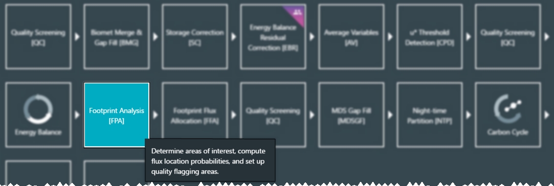
The Footprint Analysis tool allows you to explore the spatial behavior of your data set. It gives the probability that the flux came from a particular region for one particular time period (30 minutes, for example) using a two-dimensional model developed by Natascha Kljun. It can also provide aggregation of these values for different regions of interest or for different time periods.
Theory
The footprint toolbox is comprised of a set of tools based on the flux footprint analysis. Flux footprint analysis consists of a model that provides estimates of the relative contribution of each ecosystem parcel to the measured fluxes. An ecosystem parcel is a piece of surface (at the canopy top level) small enough to be considered as a “point” from the perspective of the flux measurements and of the footprint model(s). In practical term, a parcel may be an area of 1 × 1 m to 5 × 5 m, depending on the specifics of the measuring conditions.
Tovi’s footprint toolbox features the following tools:
- Research site footprint climatology
- Footprint-driven quality assessment of flux values
- Area-of-Interest driven flux imputation
- Land-use driven flux imputation
- Footprint-driven eddy covariance station evaluation
- Footprint-driven eddy covariance station design
All tools rely on the implementation of a 2D footprint model, which provides the flux footprint estimation for each time step, for which fluxes are computed, provided that the needed data and metadata are available. Each tool then uses this basic piece of information in different ways and to different purposes, as described below.
Research site footprint climatology
Using this tool, the footprint will get time-averaged footprints over defined periods of time. The user can set sorting criteria for individual footprints.
Algorithms for the footprint model
The basic, most important algorithm is the footprint model. Given a geographic domain (for example, an area of 2 × 2 km identified by the lat/long coordinates of its vertices), a 2D computational domain is created, which is intended to extend over the geographic domain. A grid is then created within the computational domain, dense enough that the resulting pixels have the size of a surface parcel. Each point of the grid is associated to a geographic location (lat/long). In the example, a computational domain of 1000 rows × 1000 columns would result in 2 × 2 m pixels, which could be an acceptable “parcel”, depending on the measuring conditions.
In Tovi, the geographic domain and the number of points (resolution of the grid) are user-selectable. However, not all combinations of extent and number of points can be allowed, because that can result in too-large computational domains. Ultimately, the limit is the computation power to calculate things on a 2D domain.
Note: All “spatial” calculations within the footprint toolbox will be performed on the 2D array representing the computational domain.
Once the computational domain has been defined, for each time step the footprint model starts from data available in the EddyPro full output and from certain metadata that needs to be provided, to compute a value of the flux footprint for each point in the computational domain. Thus, starting from a few numbers, the footprint model generates a 2D array of data, for each time step, which we will call an individual footprint. (Note that all fluxes have the same footprint, that’s why we don’t talk about the CO2 flux footprint versus sensible heat flux footprint).
Aggregation of individual footprints
Many use cases will imply making aggregations of many individual footprints, resulting in one or more footprint climatology. Aggregations will most often (if not always) mean averaging point-by-point. For example, calculating the footprint climatology over 1 full day would mean calculating the mean value of all the 48 footprints calculated for the 48 30-minute periods of a day. Again, “mean” means the average value for each point of the computational domain. In practice, you will want to perform conditional averaging, which means sorting footprint based on certain criteria, and calculating the footprint climatology for each bucket. For example, one may want to calculate the climatology during night-time and the climatology during daytime, for a month of data. Sorting criteria include (but are not limited to):
- Atmospheric stability conditions
- Wind speed
- Wind direction
- Day/night
- Seasonality
- Working/weekend days (e.g., in urban studies)
Definition and usage of Areas Of Interest
Areas of Interest (AOIs) are user-defined polygons within the geographic domain. You can define as many AOIs as you want and group two or more AOIs into a AOI group and to create multiple groups. For example, you may want to define two AOIs encompassing water bodies within the geographic domain, two encompassing forested areas and one encompassing a road passing through the geographic domain. In this case, you would define a total of 5 AOIs and group them into 3 groups, named for example, Water, Forest, Roads.
You can define the AOIs by drawing on the map and you can modify the AOI by editing, deleteing, adding points after the first drawing. Different groups can be created by choosing pens of different colors when drawing.
Once the AOIs are defined in the geographic domain, they must be mapped to the computational domain in the form of AOI masks, which are a 2D array with the same shape of the computational domain and values of True/False indicating, for each point of the grid, whether it lies within or outside the AOI. Therefore, there must be a mask for each AOI.
AOIs and AOI groups are used for making spatial aggregations of the footprint functions (whether individual or the temporally-aggregated) within meaningful areas to come up with results such as “30% of water fluxes over the summer period are coming from water bodies.”
Using the footprint analysis tool
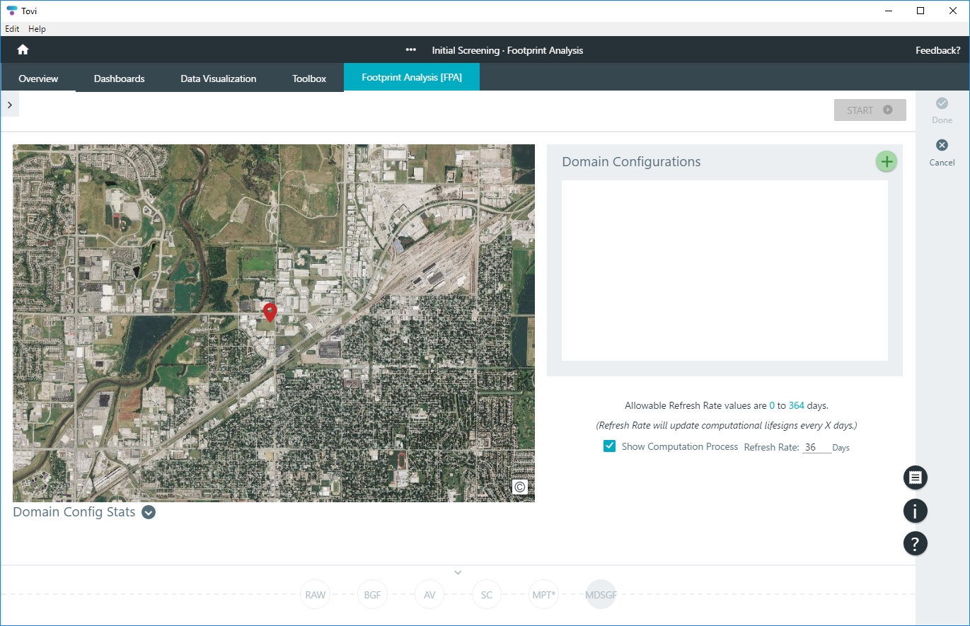
- In Overview > Analysis History, select the node to modify and click Toolbox > Footprint Analysis (FPA).
- Zoom in to find your eddy covariance station on the map. It is marked with a pin.
- Create a new Domain configuration.
- A domain configuration is a specified region with an overlaid grid for the footprint analysis. When you click the [+] button beside Domain Configuration, Tovi will open the footprint settings.
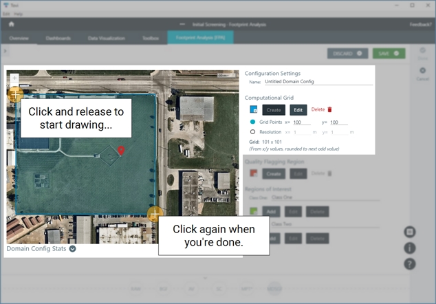
- You can either upload a GeoJSON file (see Using the GeoJSON file uploader) or configure the domain in Tovi. If you are configuring in Tovi, under Computational Grid, click New and draw around the region where you want to compute the footprint.
- Configure the grid resolution.
- By default, the grid will be 100 × 100 points, but you can select a resolution and specify the size of points within the grid. Small grid points will be higher resolution than large ones, but will take longer to process.
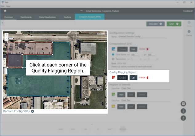
- Identify regions that you want to flag for exclusion—a walking path, pond, parking lot, or any other feature that you may want to exclude from the footprint calculations.
- These are called Quality Flagging Regions. Click Create to begin drawing these regions, and then draw one or more polygons on the map. Click to create points, and be sure to close the polygons.
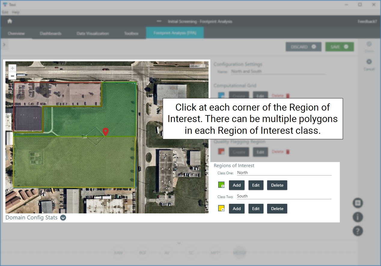
- Identify Regions of Interest—vegetation types, or any other feature that you want to explore in more detail.
- Click Add to begin drawing these regions, and then draw a polygon on the map. Click to create points, and be sure to close the polygon when you're done. Repeat this for as many Regions of Interest as needed. You can modify the polygons at any time. Name the class.
- Click Save when you're done marking Quality Flagging regions and Regions of Interest.
- Tovi will return to the Footprint Analysis home page, with the new Domain Configuration listed. You can create additional Domain Configurations if needed.
- Configure the Refresh rate and choose whether to view the process log.
- As Tovi process the footprint, you can watch the process update.
- Run the analysis: Select the Domain Configuration and click Start.

- This procedure can take some time to complete, and you cannot stop it once it is started. But, you can come back and modify the settings or create a new footprint analysis later. When Tovi is done, you'll be able to adjust the display settings and save the map as an image. Plus, now you're ready to proceed with more in-depth analysis and view the Footprint.
- Click Done to save the processing step.