Measuring gas concentrations of small samples
Authors: Liukang Xu
Correspondence: envsupport@licor.com
Published: 2020
Instruments: LI-7810, LI-7815, LI-7820, LI-7825
Keywords: small volume sample, trace gas, closed loop, open loop
Abstract
The LI-7810, LI-7815, and LI-7820 Trace Gas Analyzers are designed for high-precision and high-accuracy measurements of CH4, CO2, and N2O gases, respectively. For example, at a concentration of 2 ppm methane, the LI-7810, precision is 0.6 ppb with 1 second averaging and 0.25 ppb with 5 second averaging. Other LI-COR Trace Gas Analyzers offer high-precision measurements of their respective gases. This precision makes the analyzers ideal for long-term atmospheric methane, carbon dioxide, and nitrous oxide concentration measurements and chamber-based soil gas flux measurements.
In addition, the analyzers can be used to measure gas concentrations of small air samples when the volume of the air sample is too small for continuous flow-through measurements. As long as the air sample can be drawn into a syringe, the concentration can be measured precisely with the LI-7810, LI-7815, and LI-7820 analyzers. In addition, using small air samples allows the measurement of gas concentrations that are outside of the specified range of the instruments. In this application note we describe two methods that can be used to measure gas concentration of small air samples: closed-loop and open-loop. The examples use CH4 gas and the LI-7810 but the same procedures and considerations apply to other gases measured by LI-COR Trace Gas Analyzers.
1 | Introduction
The small volume sample kit (part number 7800-110) includes all the parts for the closed-loop and open-loop methods. The kit has the following parts:
| Description | Quantity | Part # |
|---|---|---|
| 3-way Compression Fitting | 1 | 9881-181 |
| 3-way Quick Connector | 1 | 300-07385 |
| 4-way Toggle Valve | 1 | 300-02562 |
| Silicon Septum | 8 | 300-08998 |
| Ferrule and Nut Set (1/4") | 6 | 300-15025 |
| Bev-a-line Tubing (1/8" ID) | 3.6 meters | 222-01824 |
| Hose Barb | 2 | 300-17717 |
2 | Closed-loop method
The example uses CH4, but you can follow the same procedure using CO2 or N2O and other Trace Gas Analyzers.
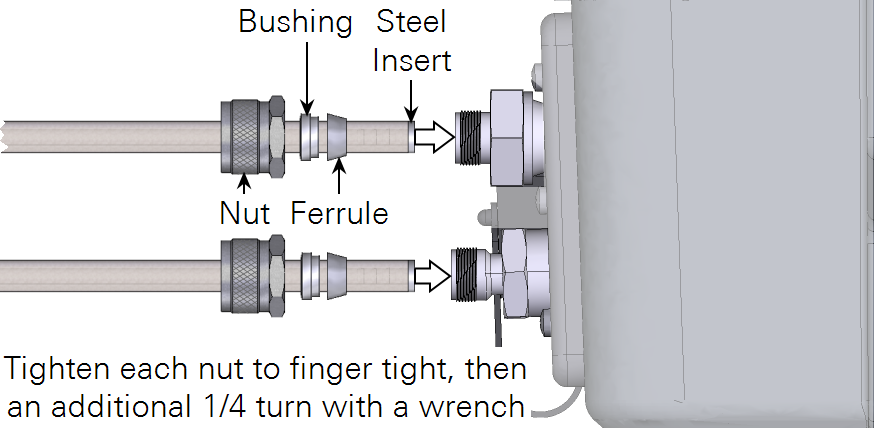
Connect tubes to the Trace Gas Analyzer (Figure 1). Insert the tube with ferrule, bushing, and knurled nut in the air inlet or air outlet. Tighten the knurled nut by hand, and then tighten it ¼ turn more with a wrench.
A 3-way T-shaped compression fitting and a 4-way toggle valve connect the inlet and outlet of the analyzer (Figure 2). The calibration gas and sample gas are injected via the septum on the T-shaped compression fitting with a precision syringe. Port 1 on the 4-way toggle valve connects to the outlet of the analyzer, and port 4 connects to the T-shaped compression fitting. Ports 2 and 5 remain open to ambient air.
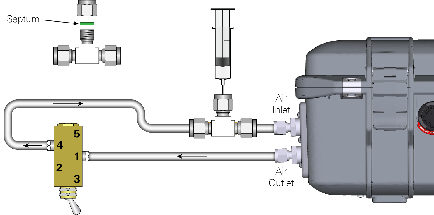
When the toggle is at the port 1 side, air is circulated from the analyzer, in to port 1, out of port 4, through the T-shaped compression fitting and back to the analyzer. The 4-way valve is used to the release air injected into the closed-loop. By switching the toggle to the port 2 side, ambient air will be pumped into the analyzer through port 5 and released back to ambient air through port 2.
2.1 | Determining the effective volume of the closed loop
Veff (cm3) is defined as the total volume of air in the closed-loop before the injection at a certain pressure and temperature. Injecting a specific volume (Vcal, cm3) of known calibration CH4 gas (CH4_cal, ppb), you will see the CH4 concentration increase from the baseline (CH4_base, ppb) to a new concentration (CH4_post, ppb). The effective volume can be estimated with equation 1b.


With ΔCH4 (ppb) being the difference between CH4_post and CH4_base. The analyzer outputs CH4 concentration data at 1 Hz (Figure 3). An average of 10 data points from a 10-second time interval is sufficient for estimating ΔCH4. To understand the procedure, ensure repeatability, and acquire a good average of Veff, you should perform this multiple times (~5 times) on the same calibration gas.

It is necessary to release the extra air injected into the loop after each sample to keep the effective volume constant between samples. Switch the toggle to the side of port 2 for 5 seconds to open the loop. Depending on the length of the bev-a-line tubing used to setup the closed-loop, Veff should be around 27-28 cm3.
If CH4 calibration gas is not available, CH4-free gas or CO2 calibration gas can also be used to estimate the effective volume using equations 1a and 1b. (Do not power on the instrument with CH4-free air.)
2.2 | Inject a specific volume of sample air
When injecting the sample (Vsam, cm3) of unknown CH4 concentration, you will see a step change in CH4, similar to the example shown in Figure 3. Once the readings are stable, a ΔCH4 (ppb) can be computed. From this, you should be able to estimate the CH4 concentration of the sample air (CH4_sam, ppb) based on the Veff, determined previously, ΔCH4, using the equation 2b.


To test the validity of equations 2a and 2b, we tried three different CH4 concentrations of calibration gases (10.747 ppm, 50.530 ppm, and 98.889 ppm) and each with three different volumes (0.25 cm3, 0.50 cm3, 0.75 cm3) with the closed-loop method. Figure 4 shows the excellent linearity between the product of ΔCH4 and the sum of Veff and Vcal and the product of the methane concentration difference between the calibration gas and the base line (CH4_cal - CH4_base) and Vcal.

The calibration line has a slope of 0.982 and R2 of 0.999. The close 1-to-1 linearity and high R-squared value demonstrates the validity and the robustness of equations 2a and 2b. One nice feature for using equation 2b is that the volume of calibration gas and sample air can be different.
When using this closed-loop method, consider the following to minimize the uncertainties in your results. First, when drawing the calibration gas or sample air into the syringe, slightly over-fill the syringe and expel some amount of air to the set-point volume just before injecting the needle into the septum.
Second, with the closed-loop configuration, the CH4 reading before or after injection might be not be as stable as you would expect. Changes can occur because the optical cavity of the analyzer operates at sub-ambient pressure of around 40 kPa. Any diffusion caused by the pressure gradient between the inside and outside of the optical cavity will likely cause small background level changes in the closed loop CH4 reading. Normally, less than one minute is needed to finish one injection measurement. If the change of CH4 concentration (ΔCH4) from the injection is larger (e.g., over 100 ppb), this small background level change can be ignored. However, if your ΔCH4 is less than 10 ppb, ΔCH4 should be corrected for the change based on the slope of CH4 just before injection.
Third, if the methane concentration of your sample air is very high, the CH4_post is approaching 50 ppm, and the volume of the sample air is already very small (~ 0.1 cm3), then an additional buffer volume can be added into the closed-loop. The buffer volume should be placed between the inlet of the analyzer and the 3-way T-shaped compression fitting. With an additional buffer volume, you would need to re-run a calibration gas to determine the new Veff. In theory, with a buffer volume of 2 liters and sample air volume of 0.1 cm3, the closed-loop method can measure the concentration of the sample air up to 100% (v/v) of methane.
Fourth, if the temperature and pressure will change during your estimation of Veff and your sample air measurements, you should normalize the volume of the calibration gas (Vcal_std) and sample air (Vsam_std) to the standard temperature and pressure (0.0 °C and 101.3 kPa) using ideal gas law.

With Psam being the ambient pressure (kPa), and Tsam being the ambient temperature (°C). Without this normalization, temperature of 10 °C difference can cause approximately 3% of error in your results, and an ambient pressure change of 1 kPa can cause approximately 1% of error in your results.
3 | Open-loop method
The example uses CH4, but you can follow the same procedure using CO2 or N2O and other LI-COR Trace Gas Analyzers.
In the open-loop method the concentration of the injected sample is determined by constructing an empirical relationship between the observed area under the curve during injection and the corresponding change in CH4 concentration. A carrier gas tank with a known CH4 concentration and a 3-way T-shaped compression fitting are needed for this method. The methane concentration of the carrier gas can be at ambient level of around 2 ppm. The carrier gas must be non-zero CH4 gas in air because the analyzer uses the CH4 absorption line for parameter optimization during the gas concentration measurement.
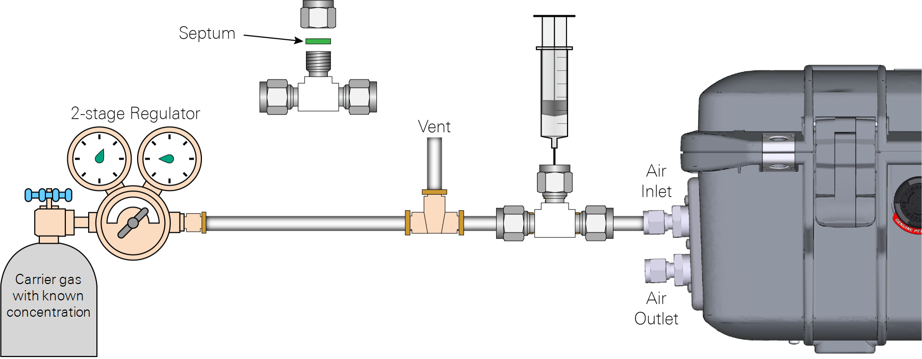
Since the analyzer flow rate is about 0.28 liter per minute (lpm), the flow rate of carrier gas from the calibration tank should be set at a rate slightly higher than 0.28 lpm. A T-shape quick connector should be installed between the carrier gas tank and the 3-way T-shaped compression fitting so excess calibration gas can be vented.
In Figure 6, we plotted the area underneath the curve from injecting 0.2 cm3 of 98.889 ppm calibration CH4 gas against the products of the methane concentration difference between calibration gas and carrier gas (CH4_cal - CH4_base) and the volume of calibration gas (Vcal).

As with the closed-loop method, it is a good idea to run this 4-5 times with the same volume and calibration gas to acquire a good average of the area underneath the pulse. Only one data point is needed to estimate the slope (α), since the calibration line must go through the origin when the concentration of calibration gas is the same as that of the carrier gas. From the empirical relationship obtained in Figure 6, we have the following equation.
4

Once you have the slope of the calibration line (α), and the area underneath the pulse from injecting sample air, the concentration of your sample air (CH4_sam) can be estimated using equation 5 below, with Vsam being the volume of the sample air.

In the example below, we used three calibration gases with three different CH4 concentrations (10.747 ppm, 50.530 ppm, and 98.889 ppm) and each with four different volumes of calibration gas (0.2 cm3, 0.4 cm3, 0.6 cm3, and 0.8 cm3) with the open-loop method. Results in Figure 7 illustrate the excellent linearity in the relationship between the area underneath the CH4 pulse from injection and the product of the methane concentration difference between calibration gas and carrier gas (CH4_cal - CH4_base) and the volume of calibration gas (Vcal).

 ).
).This result also shows the robustness and the reliability of equation 5. One advantage of using equation 5 is that the volume of your sample air does not necessarily have to be always the same. In addition, only one data point is needed to obtain the slope, α.
Because the measurement range of the methane concentration of this analyzer is from 0.1 to 50 ppm, with this method the highest methane concentration that can be measured is limited to 6000 ppm (0.6%, v/v) when using 0.05 cm3 sample air volume.
The methane analyzer outputs data at the rate of 1 Hz. From the example shown in Figure 8, one might feel that the 1-Hz output rate is not fast enough to characterize the pulse from injection. However, our testing shows the 1-Hz output rate is sufficient because the fundamental measurement frequency of the analyzer is 4 Hz. It uses block averaging to output the data at the rate of 1 Hz. In Figure 8, the pulse from 4-Hz data points is shown for comparison. As expected, the 4-Hz dataset characterized the pulse much better and smoother than the pulse from the 1-hz dataset.
However, the area underneath the pulses from 1-Hz and 4-Hz datasets are exactly the same because of the block averaging. So no additional error will be introduced with 1-Hz dataset in quantifying the area underneath the pulse.

When using the open-loop method, consider the following to minimize the uncertainties in your results. First, inject the sample into the 3-way T-shaped compression fitting quickly to minimize the technique-induced variation. Second, if the temperature and pressure will change from when you obtain the calibration line and do your air sample measurements, you should normalize the volume of calibration gas and sample air to the standard temperature and pressure.
Depending on the range of concentrations of the gas-of-interest in the air sample and the availability of a suitable carrier gas, a user can decide which method to use.