Recomputing observations
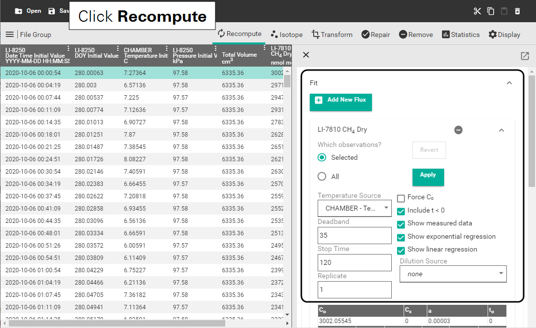
The Recompute settings allow you to use revised parameters, such as deadband, stop time, or system volume, in your flux calculations and includes tools for optimization. Any adjustments automatically recompute the flux in real time.
Note: When Which Observations is set to All or Selected and more than one is selected, no graph is displayed under Fit and Guidance is not available. Select a single observation to view the graph. If no observations are selected, any changes made in Recompute will be automatically applied to all observations.
Exploring the fit
Fit lets you change the variables used in flux calculations and observe the differences between exponential or linear fit.
Using the fit tools
- Choose whether you would like to use one of the existing fluxes or to Add New Flux.
- Add New Flux allows you to choose a new flux gas from a list of all gases measured by the device.
- Select the device and gas flux you will be recomputing.
- Select the observations you would like to work with.
- Selected refers to observations that you have selected in the Summary view. You can tell which observations you have selected, as they will be highlighted in the Summary view. You can select observations individually by clicking on them, or you can use Ctrl + click to select multiple individual observations or Shift + click to select all observations in a range.
- Update one of the variables.
- Deadband and Stop Time are common changes. The options are:
-
- Temperature Source allows you to change the source of the temperature measurement used in the flux calculation.
- Deadband is the period from complete chamber closing until steady mixing is achieved and the measurement begins. This is usually about 10 to 30 seconds but can vary and should be optimized using the Start Analysis tool (see Guidance with deadband analysis).
- Stop Time is the length of data used for the flux computation after the deadband. This can vary based on site conditions and should be optimized using the Stop Analysis tool (see Guidance with stop time analysis).
- Dilution Source lets you define the instrument that provided the water vapor measurement used in the dilution correction.
- Click Apply.
- To undo any changes you have made and return to the default settings click Revert. Revert only works on Selected observations. Any changes made to All observations cannot be undone using Revert.
Working with a single observation
If you are working with a single observation, additional features, including a fit table and chart, are available.
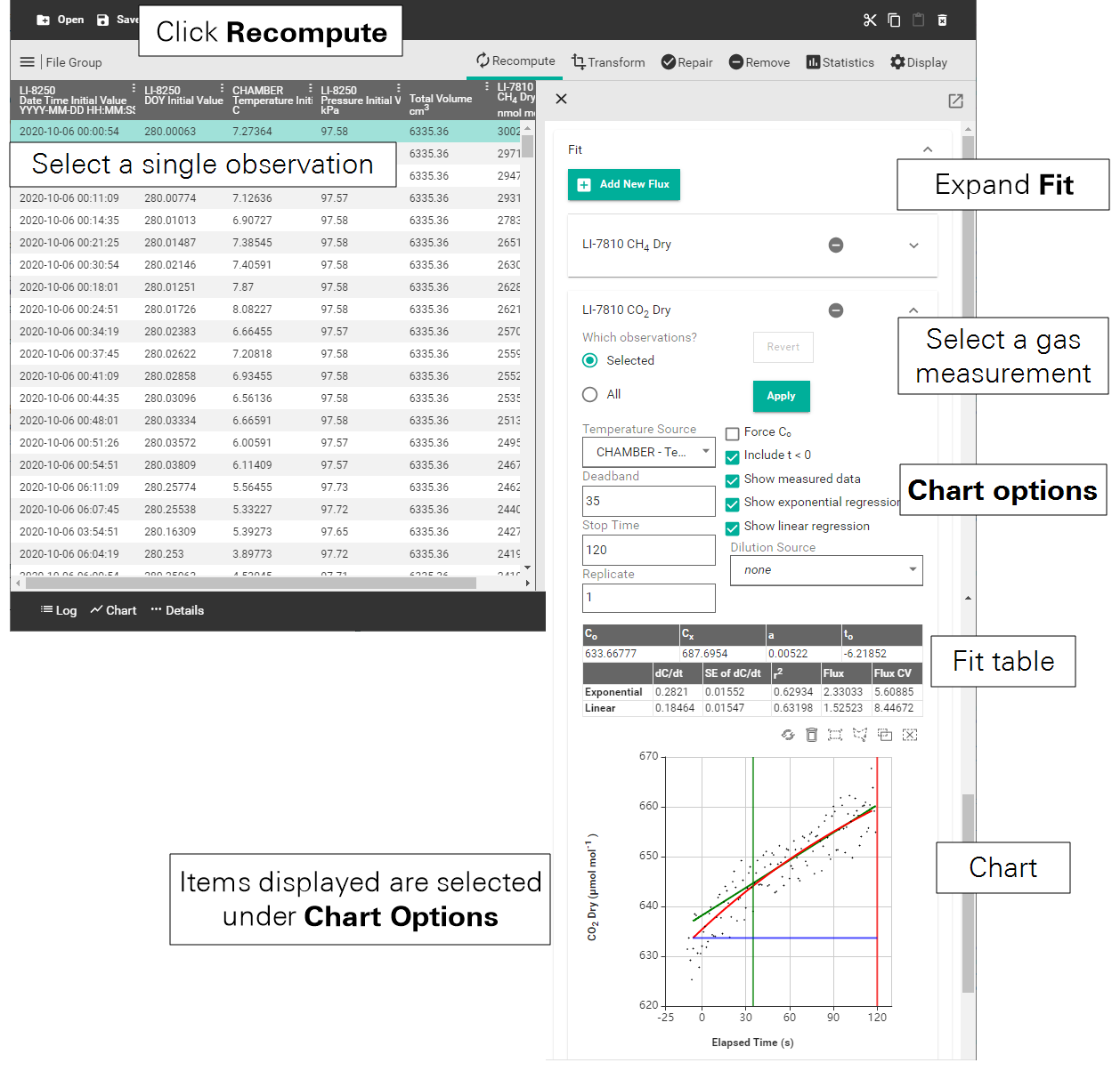
Chart Options appear when you have a single observation selected. The information displayed on the chart depends on the number of observations selected.
- Force C0 allows you to force the initial gas concentration to whatever value you want using the blue line on the chart. Usually, C0 (the starting value) is determined from the initial value. You can manually override this by checking this box and then clicking and dragging the blue line to your chosen concentration.
- Include t < 0 updates the chart to include regressions and any data points collected prior to the chamber fully closing.
- Show measured data displays the measured data points for an observation.
- Show exponential regression plots the concentration against time and exponential fit.
- Show linear regression plots the concentration against time and linear fit.
The chart gives a visual representation of the flux for a specific observation. You can adjust the deadband (green line), stop time (red line), and C0 (blue line if you have checked Force C0) by clicking and dragging them to a new location. When you release the mouse button, the data are fit linearly and exponentially with the results shown in the fit table above the chart.
The Fit table provides calculations for a number of different variables.
| Variable | Definition |
|---|---|
| C0 | Initial dilution-corrected gas measurement |
| Cx | Asymptote parameter from exponential fit |
| a | Rate constant exponential coefficient |
| t0 | Time zero |
| dC/dt | Initial rate of change in dilution-corrected gas mole fraction |
| SE of dC/dt | Standard error of dC/dt for the fit |
| r2 | r2 value for the fit |
| Flux | Calculated flux |
| Flux CV | Coefficient of variation of the fit for the flux |
Metadata
Metadata allows you to update the volume or measurements of various components to ensure you have the correct Total Volume used to calculate your soil gas fluxes. The Total Volume field itself cannot be changed by the user but must be changed by updating a device component.
To use the Metadata tool:
- Select the observations you would like to update a measurement for.
- Expand one of the device menus.
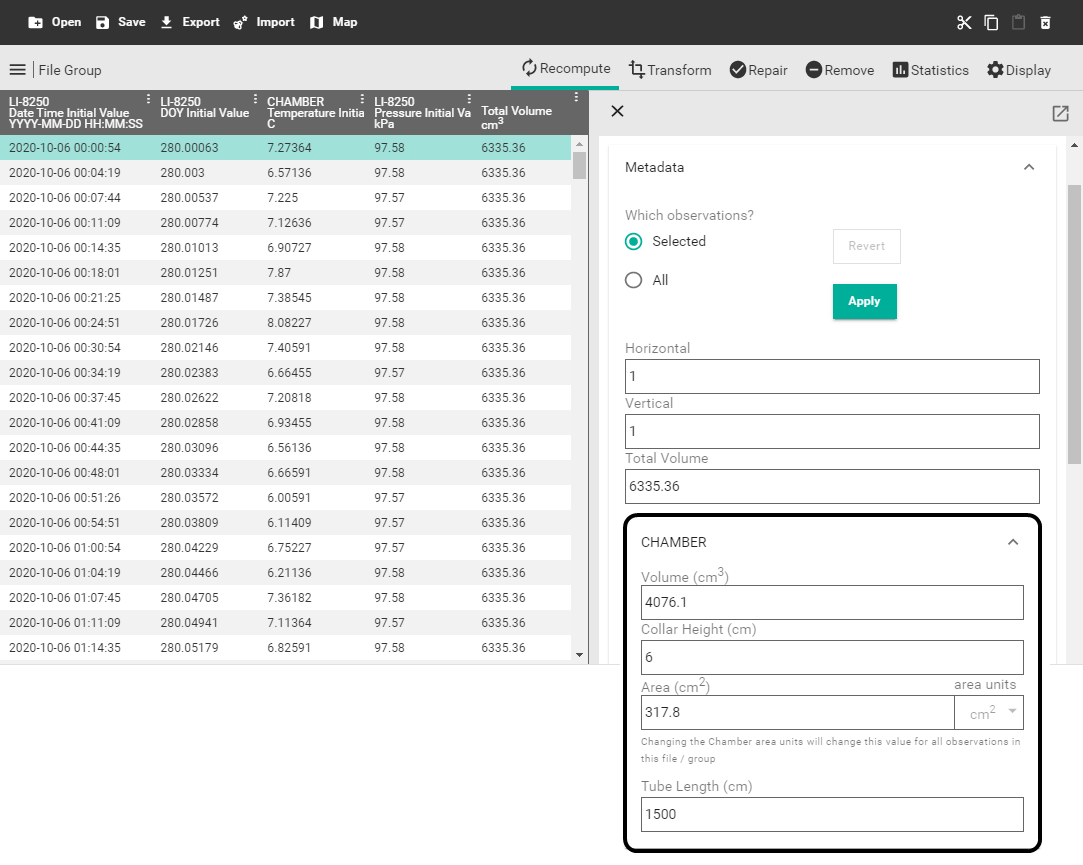
- Update one of the components, such as Collar Height, with the new measurement.
- Update any additional variables as needed.
- Click Apply.
The Total Volume will update using the new measurement data for all flux calculations on the chosen observation(s). The Revert button will return all Metadata component measurements to their original settings.
Note: The Area (cm2) field under CHAMBER includes a drop-down for area units. This drop-down allows you to change between area- and mass-based fluxes. Changing between area- or mass-based fluxes will affect the entire dataset as you may only apply a single flux type to a File Group.
Recomputing with guidance
Chamber-based closed-transient measurements of gas flux from soils involve covering an area of soil with a chamber and recording a time-series of gas concentrations inside the chamber headspace. Fluxes are computed by fitting some portion of this time series with a mathematical model. SoilFluxPro Software v5.3 presents guidance for identifying the portion of the time series for the fit over which the observed data best fit the model assumptions.
Why guidance?
The time series of gas concentrations (referred to as an accumulation curve) during a chamber-based measurement can be divided into three phases. We call them turbulence development, simple diffusion, and lateral diffusion (Figure 3‑1). In the first phase, which begins immediately after the chamber closes, the time series is dominated by the development of turbulence in the chamber. The second phase is dominated by vertical diffusion from the soil to the chamber. In the third phase, lateral diffusion begins to dominate observed changes in concentration.
The ideal window of the time series for the flux calculation includes as much data as possible from the second phase and excludes data from the first and third phases. Traditionally, this window of the time series was selected based on expert knowledge and examination of the data (often for only a subset of measurements) and applying the selection window to a broader dataset.
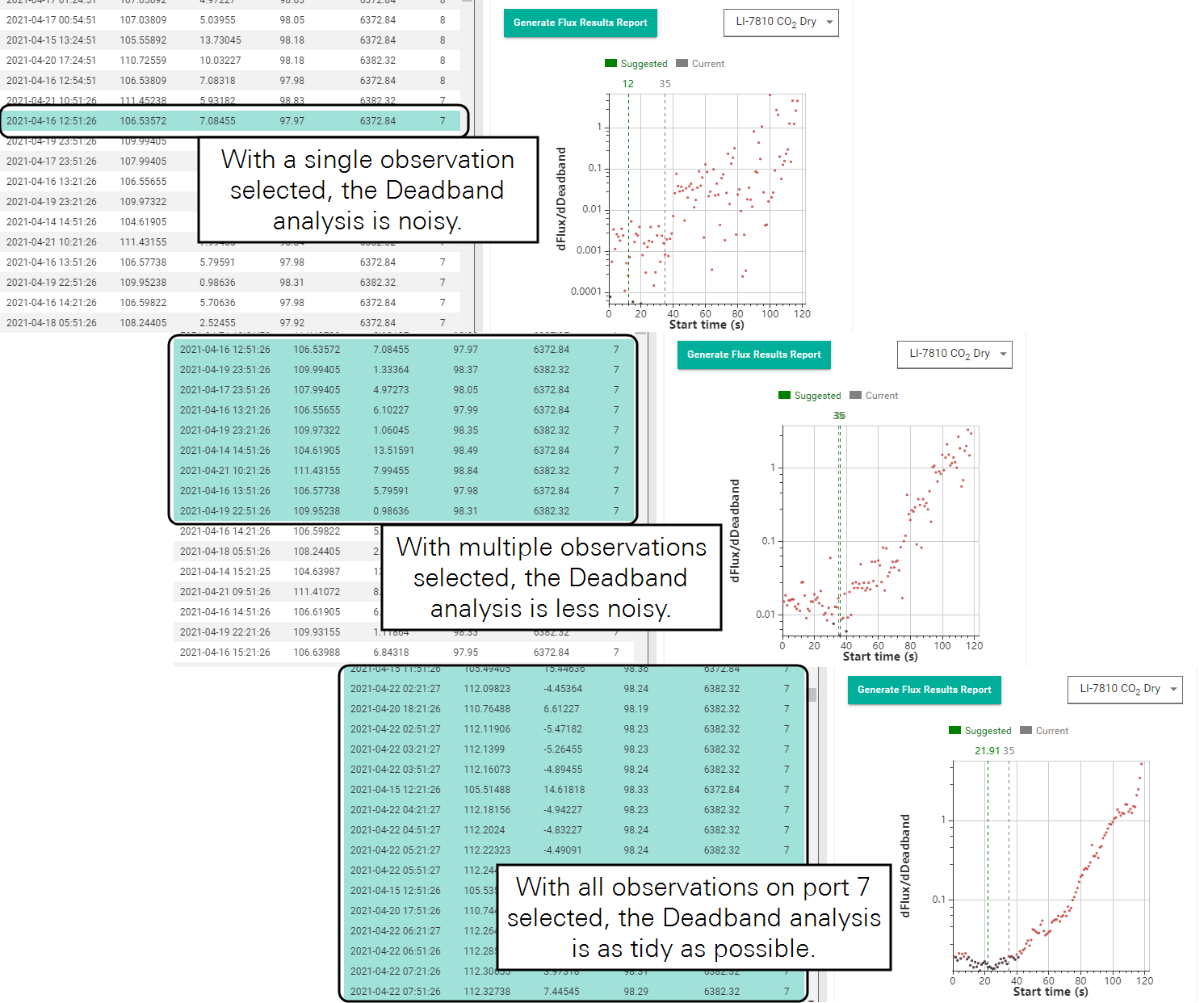
The Guidance tool removes the need for expert knowledge or subjective selection by automatically finding the window in the time series where the flux is least sensitive to the selection window. Guidance may be applied to a single flux observation, but is much more robust when applied to aggregate datasets. The benefit of this method is the ability to use an algorithm to identify the optimum window and to apply that algorithm to data from multiple observations.

Turbulence development
The first phase, referred to as turbulence development, starts at the moment of chamber closure and extends into the accumulation curve to the point at which steady state mixing has developed in the chamber and system. The length of this period is impacted by volume and geometry of the chamber, transport delays in the system, physical response times for the gas analyzers, and surface characteristics of the soil being sampled. While some of these factors are constant and well known for a given instrument system like the LI-8250, others are not and are deployment specific. They are likely to differ between each chamber placement and may change throughout the course of an experiment. Where each gas is measured by a different analyzer in the system, they are likely to differ for each gas.
Simple diffusion
The second phase is characterized by simple diffusion. After the first phase, the behavior of the accumulation curve is well described by assuming that the diffusive flux is occurring between the chamber and the soil and the change in the chamber headspace concentration accounts for most of the change in the diffusion gradient. The length of this phase is affected by the diffusive transport characteristics of the soil being measured and the absolute magnitude of the flux being measured. The starting point, duration, and end point of the second phase will likely be different for each gas measured and each chamber deployment, and will almost certainly change over the course of an experiment.
Lateral diffusion
At some point, the conditions in the chamber deviate far enough from the assumptions that the model no longer describes the behavior of the curve. At this stage, the concentration through the soil profile is being altered and some significant portion of the soil gas may be moving laterally out from under the chamber. There is a gradual transition to this phase, occurring well after the chamber closes. Both the diffusive transport characteristics of the soil being measured and the absolute magnitude of the flux being measured affect the timing of this transition. It is likely to be different for each chamber deployment and each gas measured, and will almost certainly change over the course of an experiment.
Fitting the model
SoilFluxPro fits two mathematical models to derive the flux: a linear model and an exponential model. For any model, the window of the accumulation curve that is selected for fitting has a significant impact on the reported flux. For all fits, phase 1 must be excluded. This exclusion period at the start of the observation is called the deadband. Where the linear model provides an adequate representation of the accumulation curve, the flux is less sensitive to where the deadband is set in the start of phase 2. The exponential model, however, can be quite sensitive to this and for it, the deadband needs to be set at the transition from phase 1 to phase 2. For all fitting methods, a reasonable end point in the observation must be chosen during the transition from phase 2 to phase 3. This end point is referred to as the stop time.
The exponential model provides the best test case for evaluating the sensitivities of the deadband and stop time selections. By fitting it using a deadband starting from time zero and progressively increasing the deadband, you create a time series of flux over deadband. Or conversely, the fit may be done from an arbitrary deadband to the final point in the observation moving the stop time closer to the fixed deadband to generate a curve of flux versus stop time. These two curves represent the original analysis tools in SoilFluxPro that have been available for many years.
These curves are expected to exhibit some characteristic behaviors based on the contributions of the three phases. In the case of flux versus deadband, the phase 1 region will lead to a progressively changing or erratically noisy flux from the start. As phase 2 is approached, the curve should begin to approach a constant value and as it moves past the initial part of phase 2, the flux will begin to change or become noisy.
The same general behavior should be seen for the stop time analysis as it approaches the point where phase 3 completely dominates. This is expected from theory, but rarely does the analysis for a single observation conform to this expectation. Traditionally, stop-time analysis has been done by visual inspection, relying on expert knowledge, and has typically been limited to some subset of the total dataset.
Curves of dFlux/dDeadband and dFlux/dStoptime can be generated by taking the absolute value of the change in flux per deadband and change in flux per stop time. These are used to identify the transition points without the need for visual evaluation or expert knowledge. The point where the minimum value from either set is reached marks the effective transition between phases and as such, the appropriate deadband or stop time. On a single observation basis, this curve is subject to noise in the original measurement that may make selection of the real transition points difficult. By taking the average dFlux/dDeadband or dFlux/dStoptime of many observations, the selection becomes more robust.
The selection is made by finding time of all values within some percentage of the minimum dFlux/dDeadband or dFlux/dStoptime and averaging those times to select the deadband or stop time respectively. This minimizes the effects of outliers dominating the selection, and for aggregate data, ensures the selection is made on more than one point.
The procedure can be summarized in five steps: 1) compute a set of fluxes for all deadbands or stop times from time zero to the end of the observation for one or more observations comprising a logical aggregate of observations, 2) take the absolute value of the instantaneous derivative of that set for each observation, 3) average the derivative sets across observations, 4) find the deadband or stop time for all averaged values within some percentage of the minimum value, 5) take the average of the deadbands or stop times from the minimum set.
Using guidance
In SoilFluxPro 5.3, the Guidance feature can operate on a range of observations instead of on a single observation, as in previous versions. With multiplexed data, it is useful to apply guidance by port (chamber), for example. Guidance will give advice on two aspects of the data: Deadband and Stop Time.
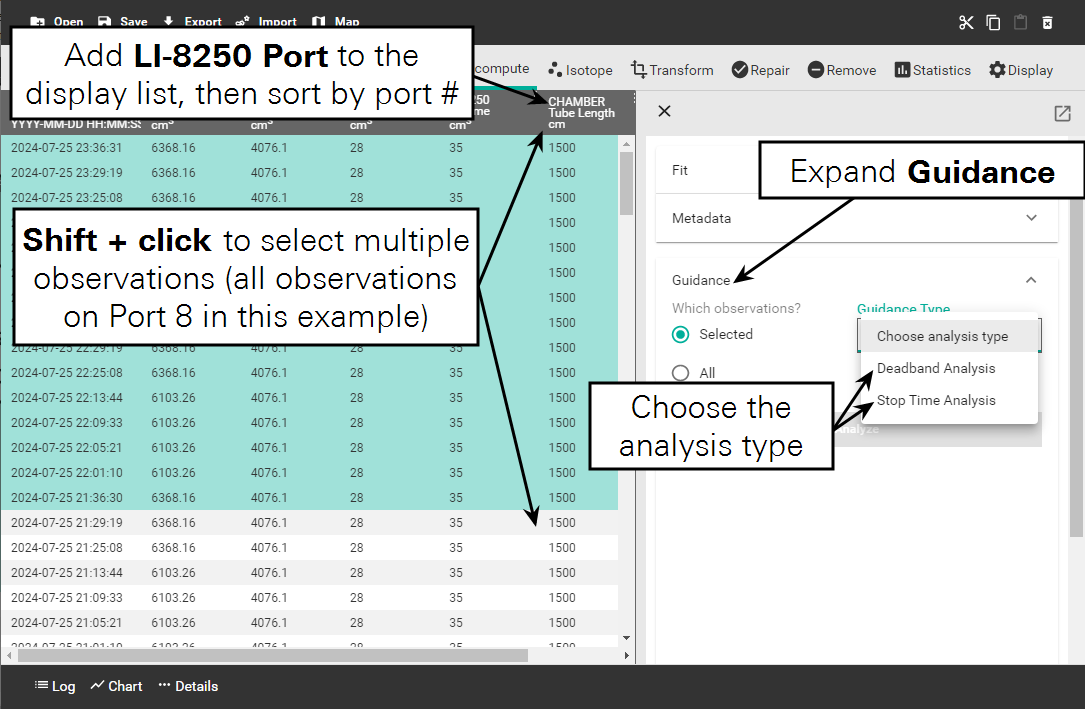
Guidance with deadband analysis
Deadband analysis is designed to operate on multiple observations or single observations. Figure 3‑3 shows how to start deadband analysis on observations from Port 8.
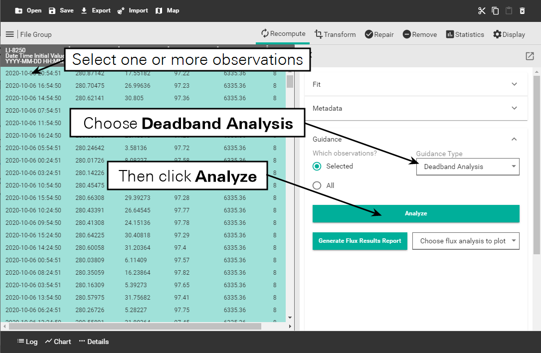
The analysis is computationally intensive - it may take a moment. After the analysis is complete, you can choose a specific flux analysis to plot.
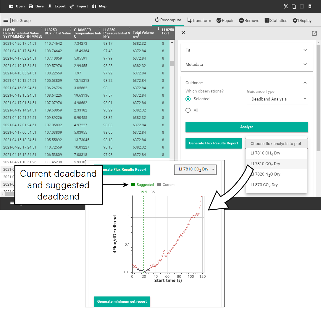
The plotted results show the current deadband, and the suggested deadband. If they are different, you recompute the results with the suggested deadband.
Guidance with stop time analysis
Stop time analysis optimizes the third phase of the observation. Optimizing the stop time ensures that the computations do not include the effects of lateral diffusion.
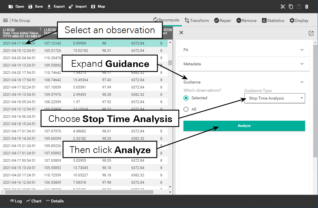

The plotted results show the current stop time, and the suggested stop time. If they are different, you recompute the results with the suggested stop time.
Deadband flux report
The Deadband Flux Results Report presents a table for current and suggested deadbands, if you want the details as a table. You can also read values used for purple points in the plot by clicking Generate minimum dataset report.