FV2200 duplicates the LAI computation done in the LAI-2200C console (LAI‑2000 Method), and also provides some alternatives: the Lang Method, Ellipsoidal Method, and Constrained Least Squares Method. These are described below.
There are some points to remember when interpreting these results:
- The “L” in LAI (Leaf Area Index) is traditional, and not necessarily a fact. Anything that blocks light will be included in the result: branches, stems, animals, etc. Thus, “Foliage Area Index” is a better way to think of this.
- LAI could be foliage area index (m2 foliage/m2 ground), or foliage area density (m2/m3) canopy. It is the path lengths (Dist[*]) that determine which units are appropriate. For standard path lengths (Horizontal Uniform model), LAI is foliage area index. For any other path lengths (Isolated Canopy, Measured Distances, and Isolated Canopy, Computed Distances), LAI should be interpreted as foliage density.
- The LAI values include a correction (log average transmittances) for clumping. Thus, especially if narrow view caps were used, measured LAI is closer to L (true LAI) than Le (effective LAI). If you want Le, multiply LAI by ACF, the apparent clumping factor.
LAI‑2000 Method
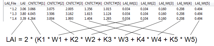
LAI is computed from (see Theory for the derivation):
G‑1

where L is the leaf (all light blocking objects) area index (LAI),  is the mean contact number for the ith ring (CONTACT#[*]), and Wi is the weighting factor for the ith ring (LAI_W[*]).
The mean contact number is a function of the transmittance and the path length Si (DIST[*]). For n Above/Below pairs of observations,
G‑2

Weighting factor Wi is computed from
G‑3

where  is the mean zenith angle and
  is the ring width (radians) associated with ith ring. Values for
  are given in Table G‑1 below. The weighting factors are normalized to sum to 1.0, so when one or more rings are masked, the remaining weighting factors increase.
|
Ring |
Width (°) |
Weighting Factor |
|---|---|---|
|
1 |
12.2 |
0.041 |
|
2 |
12.2 |
0.131 |
|
3 |
11.8 |
0.201 |
|
4 |
13.2 |
0.290 |
|
5 |
13.2 |
0.337 |
Lang Method
A simple method of computing LAI from the slope and intercept of a plot of contact number vs. angle was proposed by Lang (1987).
G‑4

where Llang is leaf area index (LangLAI), m is the slope and b is the intercept of contact number (CNTCT#[*]) plotted as a function of angle (in radians). LangLAI can be added to views or viewed in the “All Values” tab of any data file.
Ellipsoidal Method
Another method of inverting gap fraction data is to use an ellipsoidal-based description of leaf angle distribution. Refer to Norman and Campbell (1989), and Campbell (1986).
Variables computed with the Ellipsoidal Method include:
EllipLAI – LAI (or foliage density) obtained from the ellipsoidal distribution method.
EllipMTA – Mean Tilt Angle obtained from the ellipsoidal method.
EllipX – The ratio of horizontal to vertical radii of an ellipsoid whose surface area fractions describe the foliage angle distributions in the canopy.
These variables can be added to views or viewed in the “All Values” tab of any data file.
Constrained Least Squares Method
An alternative method of inverting gap fraction data is that of constrained least squares. Refer to Norman and Campbell (1989) and Perry et al. (1988). The outputs associated with this method are listed below:
CLS_LAI – LAI (or foliage density) by method of the constrained least squares.
CLS_c – The smallest constraint that yields all positive area fractions.
CLS_LAD[*] – foliage angle distribution. The angle classes are 9°, 27°, 45°, 63°, and 81° (90 divided evenly by 5). If one or more rings are masked, there will be fewer angle classes.
CLS_MTA – Mean Tilt Angle based on the distribution (S).
CLS_Mu, CLS_Nu – Mu, Nu of the Beta distribution (Goel and Strebel, 1984).