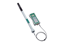
The LAI-2200C measures the probability of seeing the sky when looking up through a vegetative canopy in different directions. These measurements essentially contain two pieces of structural information about the canopy: 1) the amount of foliage in the canopy and 2) the foliage orientation. This section describes the details of how the LAI-2200C extracts this information from its measurements.
Calculations
As a beam of light passes through a plant canopy, there is a certain probability that it will be intercepted by foliage. The probability of interception is proportional to the path length, foliage density (area of foliage per volume of canopy), and foliage orientation. If foliage elements are small compared to the overall canopy, and they are randomly distributed in the sensor view, then it is well known that a beam of light from zenith angle θ has a probability of P(θ) of non-interception:

where G(θ) is the fraction of foliage projected toward θ, µ is foliage density (m2 foliage per m3 canopy volume), and S(θ) is path length (m) through the canopy at angle θ. Miller (1967) gives the exact solution for µ as

Foliage Density and Leaf Area Index
In a horizontally large, homogeneous canopy, path length, S(θ) is related to canopy height h by
J‑3

In such a canopy, the relation between leaf area index L and foliage density µ is
J‑4

Substituting these into (10-2) yields


Thus, we can use a common formula J‑7 for computing either L or μ: For L, we use S(θ)=1/cosθ (height h does not matter because it cancels out of equation J‑5, and for computing μ we use actual values of S(θ). The difference between L and μ is driven by S(θ).
Clumping
When multiple observations of P(θ) are available, there are two ways they can be combined: The values of P(θ) can be averaged:

or the values of lnP(θ) averaged:

Equation J‑7 will account for clumping (on spatial scales larger than the field of view of the sensor), but equation J‑6 is appropriate for determining effective leaf area index Le, which by definition must ignore clumping.
The LAI-2200C computes both of these, and uses equation J‑7 for its reported leaf area index value L, and the ratio of equations J‑6 and J‑7 for computing Ωapp, the apparent clumping factor (Ryu et al. 2010).
J‑8

Effective leaf area index, Le, can be computed by
J‑9

Foliage Orientation
Once L or µ is determined from equation J‑1, equation J‑2 can be solved for the orientation function G(θ).
J‑10

Figure J‑1 shows the theoretical values of G(θ) for an ideal canopy whose foliage is random both in position and azimuthal orientation, but inclined at a fixed angle. Curves for ten different foliage inclination angles are shown.
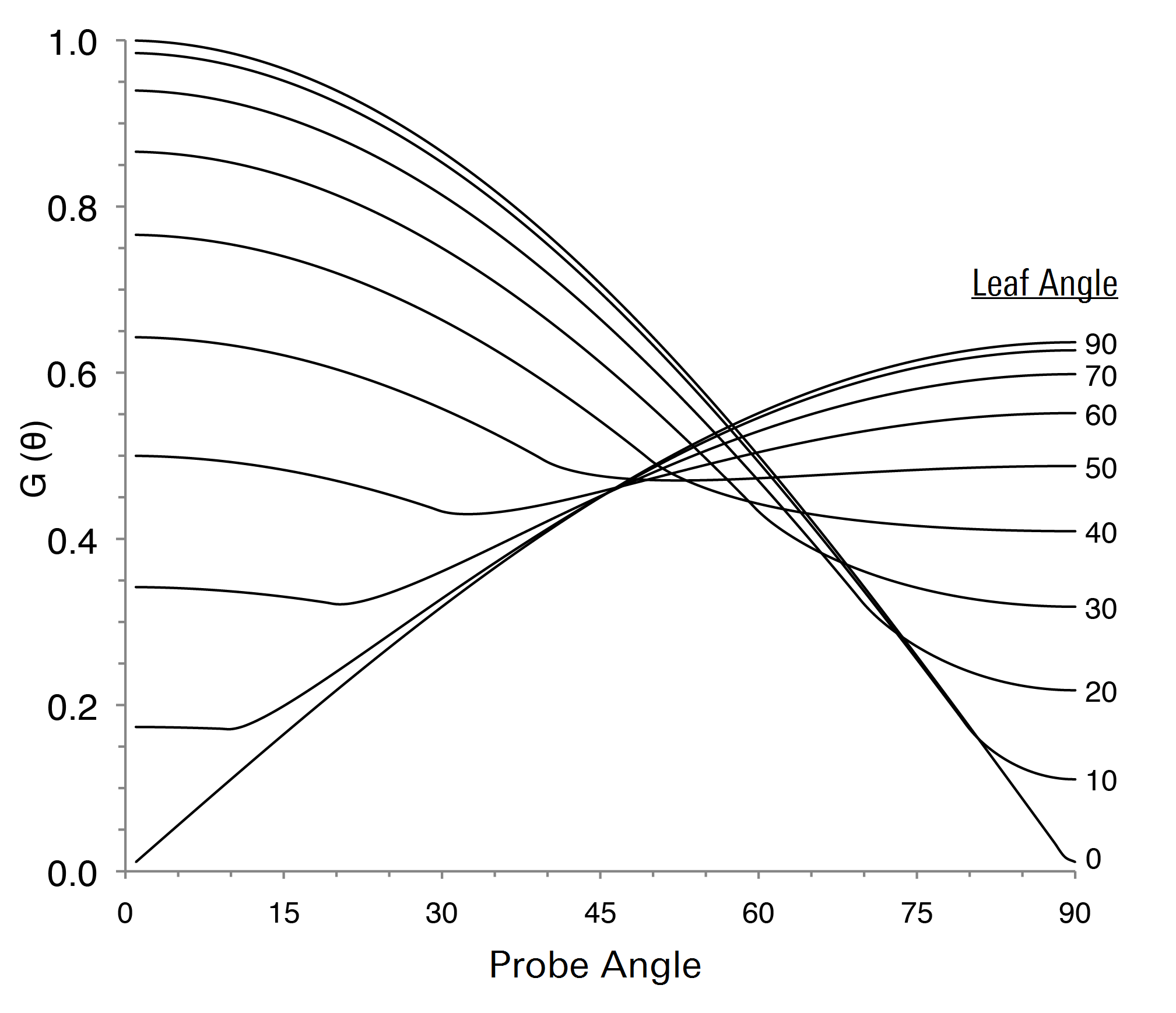
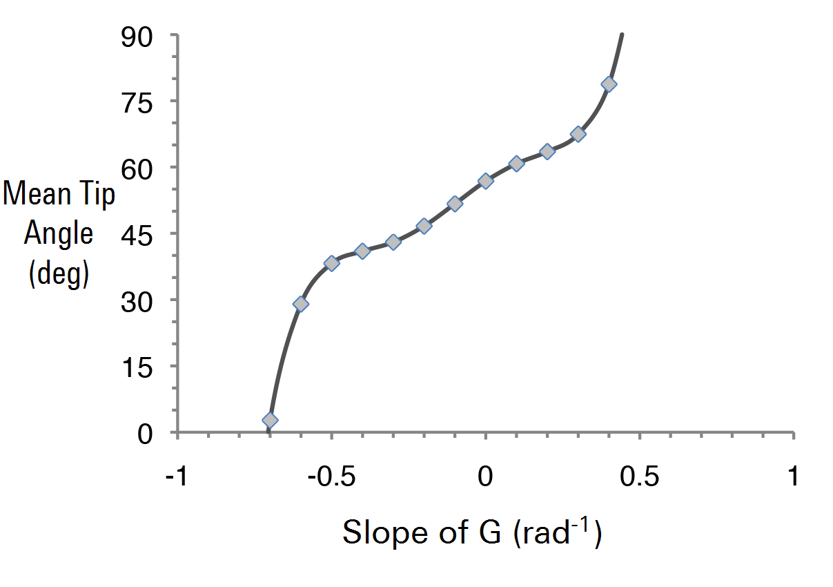
The (rad-1) LAI-2200C calculates foliage mean tilt angle  after the manner of Lang (1986), using an empirical polynomial relating inclination angle to the slopes of the idealized curves between 25° and 65° (data in Table J‑1, plot in Figure J‑2).
| MTA (degrees) | Slope | MTA (degrees) | Slope | |
|---|---|---|---|---|
|
1 |
-0.6964 |
50 |
-0.1547 |
|
|
10 |
-0.6859 |
60 |
0.1180 |
|
|
20 |
-0.6546 |
70 |
0.3164 |
|
|
30 |
-0.5855 |
80 |
0.4131 |
|
|
40 |
-0.4105 |
89 |
0.4431 |
Implementation Algorithms
In this section, the subscript i refers to optical sensor rings (i=1…5), and the subscript j refers to observational pairs (j=1…Nobs). Bij is the jth below-canopy observation, ith ring, and Aij is its corresponding above canopy reading.
AVGTRANS
The average probability of light penetration into the canopy is computed by
J‑11

The 5 values of  are labeled AVGTRANS in the LAI-2200C data file.
GAPS
The probability of light penetration based on averaging the logarithms of transmittance for the ith ring is computed from
J‑12

The values of Gi are labeled GAPS in the data file.
LAI and CNTCT#
The leaf area index L for the file, labeled LAI, is computed from
J‑13

where
J‑14

and
J‑15

Ki is sometimes called the contact number, and is reported with the label CNTCT# in the data file. For further explanation of Wi, see Weighting Factors, below.
ACF and ACFS
An apparent clumping factor for each ring, labeled ACFS in the LAI-2200C data file, is computed from
J‑16

A total apparent clumping factor, Ωapp, labeled ACF in the data file, is computed from
J‑17

SEL and STDDEV
Standard error Lse of the leaf area index value is reported as SEL, and is computed from
J‑18

where Lj is the leaf area index calculated for an individual A/B pair
J‑19

where Kij is the contact value for the pair.
J‑20

The standard deviation  of the contact numbers is reported as STDEV, and computed from
J‑21

MTA
Mean Tilt Angle α̅f is the average inclination of the foliage in degrees from the horizontal (0=flat, 90=vertical), and is computed from a 5th order polynomial α(m):
J‑22

where
a0=56.81964
a1=46.84833
a2=-64.62133
a3=-158.69141
a4=522.06260
a5=1008.14931
The value of α(m) is constrained so that 0≤α(m)≤90. The independent variable m is the slope of the mean contact numbers (K) plotted against ring angle θ in radians.
J‑23

SEM
Standard error of the mean tilt angle is estimated from
J‑24

where mse is the standard error of the slope m. When m > 0, we use (m-mse); otherwise, we use (m+mse).
DIFN
Diffuse non-interceptance D is the fraction of sky radiation that will penetrate the canopy, averaged over the hemisphere (Norman and Welles, 1983). Note: this is computed from  not
not  .
.
J‑25

where
J‑26

This value is reported as DIFN in the data file. FV2200 makes a related computation (Dsky, labeled DIFN_SKY), that is weighted by sky brightness distribution based on the A readings.
J‑27

where Ai is the average of the NA above canopy readings in the file.
J‑28

Weighting Factors
The weighting factors for LAI and DIFN work out to be (when no rings are masked):
| θi | dθi | Wi sinθdθ |
W'i sinθcosθdθ |
|---|---|---|---|
|
7 |
12.2 |
0.041 |
0.033 |
|
23 |
12.2 |
0.131 |
0.097 |
|
38 |
11.8 |
0.201 |
0.127 |
|
53 |
13.2 |
0.290 |
0.141 |
|
68 |
13.2 |
0.337 |
0.102 |
When a ring is masked (excluded from the computations), its weighting value is set to 0. This will increase the weighting of the remaining rings, since their sum must be
J‑29

and
J‑30

The values of Wi are available on the FV2200 as the LAI_wt, and the values of W’i are shown as DIFN_wt.
Alternative Methods
Gap fractions have been measured using fisheye photographs (Anderson, 1971; Bonhomme and Chartier 1972), by traversing a sunward-pointed sensor beneath the canopy (reviewed by Ross, 1981; Lang et al. 1985; Perry et al. 1988), by linear light sensors (Walker et al. 1988), and by pushing metal probes through the canopy (Warren Wilson, 1959).
See Norman and Campbell (1989), Welles (1990), Welles and Cohen (1996), Gower et al. (1999), Machado and Reich (1999), de Jesus et al. (2001), Mussche et al. (2001), Breda (2003) Hyer and Goertz (2004), Keane et al. (2005), Garrigues et al. (2008) for additional reviews and comparisons.
Mathematical techniques for deducing foliage density and angle distribution from measurements of gap fraction (or contact frequency) have been presented by many authors, including Warren Wilson (1959), Miller (1963, 1967), Philip (1965), Ross (1981), Anderson (1984a, 1984b), Lang (1986, 1987), Lang et al. (1985), Perry et al. (1988), and Norman and Campbell (1989).
Scattering Correction
One of the traditional underlying assumptions of the LAI‑2000 and LAI-2200C has always been that foliage absorbs all the radiation in the waveband seen by the sensor (320-490 nm). Starting with version 2.0, FV2200 allows this assumption to be set aside, and provides a model (Kobayashi et al, 2013) for correcting measurements for the radiation reflected and transmitted by the foliage.
How Scattering Correction Works
The algorithm that FV2200 uses for correcting for scattering goes something like this:
- Compute gap fractions. From the measured gap fractions, calculate a first guess of leaf area index (LAI) and leaf angle distribution (LAD).
- Predict the scattering effect on gap fractions. Run the Kobayashi model to predict the error that an LAI-2200C would make in a canopy based on LAI, LAD, and the other scattering correction inputs (leaf properties, sky brightness distribution, etc.). The model is a one-dimensional, multi-layer model, having foliage properties that you have specified. Foliage orientation, clumping, and total LAI is based on Step 1.
- The model propagates beam and diffuse radiation through the layers, and predicts fractional irradiances on sunlit and shaded leaves in each layer. It then predicts the view that the LAI sensor, and the bottom of the canopy, has of the sunlit and shaded foliage throughout the model, and the resulting radiation errors each ring of a B reading would have.
- Subtract the scattering effect from gap fractions. The gap fractions are then adjusted to remove the predicted scattering effects.
- The adjusted gap fractions are used to compute a new LAI and LAD. If they have not changed, the process is done. Otherwise, it’s back to step 2 with the adjusted gap fractions.
This process usually takes 4 or 5 iterations.
Required Inputs for the Scattering Model
The scattering model uses the following inputs:
- LeafRho: Average foliage reflectance in the blue (230-490 nm waveband).
- LeafTau: Average foliage transmittance in the blue.
- SoilRho: Surface reflectance beneath the canopy in the blue.
- SolarZen: Solar zenith angle (0° = overhead, 90° = on horizon).
- SolarAzm: Solar azimuth angle (0° = North, 90° = East, etc.).
- SkyViewCap: The azimuthal view size of WideSky values (e.g. 270°).
- AViewCap: The azimuthal view size of ASky values (e.g. 45°).
- AViewAzm: The azimuthal direction of ASky values (0° = N, 90° = East, etc.).
- FBeam: The fraction of the total incident radiation from the sky that is direct beam, in the blue.
- WideSky: The 5 ring values of sky brightness using the SkyViewCap.
- ASky: The 5 ring values of sky brightness using the ASky Cap.
Scattering Properties
The three values for average vegetative reflectance, transmittance, and the surface beneath the canopy (LeafRho, LeafTau, and SoilRho) should be for the 320-490 nm (blue) waveband. The values could come from spectroradiometric measurements integrated over this waveband, or from a radiometer sensitive in that waveband.
Kobayashi et. al. present a technique for using the LAI‑2x00 optical sensor (wand) and a reference panel to determine leaf reflectance (LeafRho) and transmittance (LeafTau) values. To use this method, follow Procedure 2.14 - Measuring Leaf Transmittance and Reflectance. A lens cap with a small hole at the center (1.27 mm in diameter) was attached to the optical sensor. They also used a white halon diffuse reflectance standard panel (25 cm x 25 cm and 99% reflectivity).
Sky Brightness Properties
Both WideSky and ASky have the following constraints:
- They need to be made with an unobstructed view of the sky.
- They should be made with the same wand.
- The wands making the measurements should be using the factory calibration values. This is the calibration that relates one ring to another. With this calibration, all of the sensor’s rings will read the same in a purely isotropic environment. This (WideSky and ASky) is the one time in LAI-2200C processing that the rings of the sensor are NOT treated independently, and the factory isotropic calibration is needed.
Derivation of Formulae for Determining # of B Readings
The guideline presented in Chapter 4 for determining the number of B readings (How Many B Readings? ) comes from the following analysis:

where M is the true mean of a population, m is the mean of a sample of that population, t(n) is the value of the t distribution (ignoring sign) for a 5% probability, and E is the standard error of m. We rewrite equation J‑31 in terms of an acceptable uncertainty  :
:
J‑32

Since standard error E is standard deviation D divided by the square root of the number of samples n, we can express  as:
as:

To solve equation J‑33 for sample size n, we find a functional relationship for t(n) by fitting a curve to the form

and find a = -0.11528, b = 0.060798, and c = 2.9817. Substituting equation J‑34 into J‑33 and solving for n yields

where
 and
and  .
.
As a practical matter, the term  can be determined by a “trial measurement” with the LAI-2200C using some number of B readings. These readings should be a fair representation of the diversity of the foliage density. Given LAI, SEL, and SMP, the
  term can be computed from
J‑36

Table J‑2, from equation J‑35, predicts the number of samples necessary for a 95% confidence that a sampled mean is within some error  of a population mean.
|
|
n |
|
|
n |
|
|
n |
|
0.2 |
2 |
1.2 |
8 |
2.2 |
19 |
||
|
0.4 |
3 |
1.4 |
10 |
2.4 |
22 |
||
|
0.6 |
4 |
1.6 |
12 |
2.6 |
25 |
||
|
0.8 |
5 |
1.8 |
14 |
2.8 |
28 |
||
|
1.0 |
7 |
|
2.0 |
16 |
|
3.0 |
30 |


Table D‑1 is in terms of SEL and LAI, rather than D and m, and is based on a sample of 6 (SMP) with  = 0.1.