This section includes practical considerations for data collection procedures and guidelines for collecting data under a variety of conditions.
Guidelines for Getting Good Data
Collecting reliable data with the LAI-2200C depends on having a protocol that is appropriate for the canopy of interest and suitable for the measurement conditions. For any A or B readings that are used as a pair, the view cap must be the same size, the optical sensor (wand) must view the same part of the sky, and the view cap must cover the same part of the sensor (this only applies if the same sensor is used for both A and B readings). These and other considerations are discussed below.
Where to Measure?
A Readings
In general, A readings should be made as closely as possible to B readings, both in time and space; however, under certain conditions and with the appropriate protocol, this is not essential to acquiring good data.
In some situations, especially in forest canopies, it may be impossible or impractical to record A readings near the B readings. In these situations, it is best to use two optical sensors (see Operation: Two Sensors, One Control Unit), with one sensor positioned above the canopy or in a clearing, logging data automatically. Additional suggestions are in Canopy Types.
B Readings
It is best to consider a sampling protocol that is designed for the canopy type that is being measured. The best protocol for measuring a short homogeneous canopy (such as a grassland) may not be the best protocol for measuring a row crop (and it certainly will not be the best protocol for measuring a tall heterogeneous canopy). Guidelines for measuring specific canopy types are presented in Canopy Types.
One approach to collecting B readings is to make measurements equally spaced along one or more transects under the canopy. Alternatively, measurements can be made at randomly chosen locations in the study area, though practical considerations periodically make this difficult. Predetermined sample locations may violate the guidelines for usage and require adjustments to the sample location in order to collect valid data. For example, avoid making measurements with a leaf immediately above the sensor, because one leaf may block the entire view of the center rings. At the larger zenith angles, when foliage is beside the sensor rather than above it, an individual leaf blocks much less of the view. The section called Foliage Size, provides detailed guidelines for minimum distances and the theoretical justifications. Refer to Ross (1981) for guidelines used for fisheye photography.
How Many B Readings?
When determining the proper number of B readings, first consider the ground area over which the computed LAI is to be valid: An entire field? Part of a field? A small plot? Second, what fraction of this area does one B reading represent? As a rule of thumb, consider each B reading to represent a sample of the canopy that is cylindrical (or some fraction of a cylinder if a view cap is used) with a radius roughly equal to the canopy height (the potential view of the sensor is larger than this, but the effective range is reduced by foliage). Thus,
D‑1

where A is the ground area represented by the sample, f is the view fraction (0.75, 0.5, 0.25, or 0.125 for the 270°, 180°, 90°, and 45° view caps respectively), and H is canopy height. For example, one B reading with no view cap (f=1) in a canopy 5.0 m on a side and 1.0 m tall is a sampling of approximately 3 m2, or 12% of the total ground area. If that same canopy were only 0.2 m tall, then one B reading would represent only 0.5% of the ground area. Thus, canopy height is a very important consideration.
Another consideration is the variability of the density of the foliage in the plot. A homogenous canopy would require fewer B readings than a heterogeneous one. Table D‑1 provides guidelines for determining the proper number of B readings. See Derivation of Formulae for Determining # of B Readings for the derivation.
This simple procedure is used to determine the number of B readings necessary for 95% confidence that the true LAI mean is within ±10% of the measured LAI.
- Make an LAI reading based on 6 B readings. Be sure to include both the thinnest and densest parts of the canopy.
- Divide the Standard Error of LAI by LAI (SEL/LAI)
- Use Table D‑1 to determine the number of B readings.
| SEL/LAI | #B Readings | SEL/LAI | #B Readings |
|---|---|---|---|
| 0.01 | 2 | 0.06 | 11 |
| 0.02 | 3 | 0.07 | 13 |
| 0.03 | 5 | 0.08 | 16 |
| 0.04 | 6 | 0.09 | 19 |
| 0.05 | 8 | 0.1 | 23 |
Using View Caps
Use the 270° view cap to hide the operator from the sensor any time measurements will be made with the operator potentially in the field of view. No view cap is needed if the operator is very careful to block exactly the same portion of the sensor’s field of view for both A and B measurements, but it is simpler to use the view cap.
In general, any object that is common to both the A and B readings will not affect the LAI computation. Thus, one could measure the LAI of grass beneath a tree if the A and B readings are in close proximity so that the tree occupies the same portion of the sensor’s view for both A and B readings.
Here is a summary of reasons to use a view cap:
- To remove the sun from the sensor’s view
- To remove the operator from the sensor’s view
- When sky brightness is very non-uniform
- When there are significant gaps or clumps in the canopy
- To reduce the required plot size
- To reduce the required clearing size for above-canopy readings in a forest
There are times when it is preferable to use the 180° or 270° field of view instead of a narrow one:
- To avoid loss of signal near twilight or under very dense canopies
- If the goal of the measurement is Le (effective LAI), not L (true LAI).
Be very careful that the A and B sets of readings are made with the sensor(s) viewing the same region of sky without rotating the view cap on the sensor. This is because there are usually slight azimuthal variations in the sensitivity of the optical sensor’s detector, especially on the outer ring.
When using the view cap to block the sun, it is good practice to shade the entire lens from the sun, to prevent light reflected from the surrounding view cap structure from influencing the readings. Usually it is only the 5th ring that responds to such reflections.
Measuring on Slopes
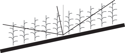
When making measurements on sloping terrain, there are a couple of strategies that can be employed. One method is to hold the optical sensor parallel to the ground rather than level. Make sure that all associated A and B readings are made with the sensor tilted at the same inclination and pointed in the same compass direction.
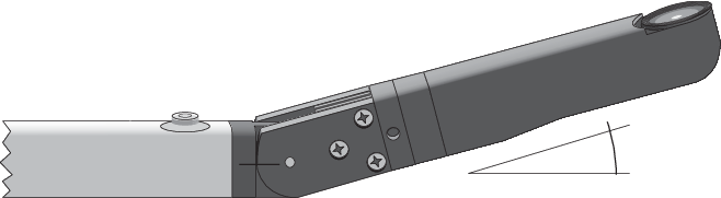
One way to ensure that the sensor is held at the same inclination for each reading is to mount the bubble level on the handle rather than the sensor. Fix the hinge at an angle that permits the handle to be held level while the sensor is held at the desired inclination. Mark the two pieces at the hinge so that this angle can be reset easily (see Figure D‑2).
If it is impossible to incline the “above” and “below” sensors at the same angle when measuring on a slope, the effects can be minimized by using a 45° view cap, and orienting the sensor for B readings along the contour (looking neither uphill nor downhill). The A readings need to be taken at the same compass direction as the B readings.
Another way to minimize the effects of the slope is to mask out the outer two or three rings in the analysis, either before (Procedure 2.10 - Excluding Rings from Analysis - Console or after (Procedure 3.5 - Excluding Rings from Analysis - FV2200) data collection.
Sloping ground has some implications for scattering corrections if you are measuring with the sensor parallel to the ground (first method). This is discussed in K Records and Sloping Terrain.
Bad Readings
Theoretically, B readings should always have lower values than A readings. In very sparse foliage they will be very close, and in large gaps where no foliage is seen by the sensor, they will be identical. But that is only in theory.
As a practical matter, a B reading may exceed the value of its A reading for any of the following reasons:
- Changing sky conditions
- Normal measurement variation
- Operator error (A and B out of sequence)
- Making B readings in sunlit foliage
A B reading is “bad” if one or more of the rings has a value that exceeds its associated A reading, so that the transmittance for that ring is greater than 1.0. If this is due to operator error or changing sky conditions, it would be good for the operator to be alerted so that the measurement can be started over. But if a reading is bad simply because of sparse foliage and normal fluctuations, it would be nice for the console (control unit) to overlook the slight discrepancy and proceed using a value of 1.0 for the transmittance(s) of the offending ring(s).
To determine this setting, go to MENU > Log Setup > Transcomp > and scroll down to Bad Readings. Select one of the settings described below (press OK to save the setting).
Skip: When a transmittance greater than 1.0 is found, that B reading is ignored in the calculation. The offending record is still stored in the file, however. You will know that a bad reading occurred if the number of B readings is larger than the sample size in Logging Mode (see Logging Mode). Skip should be used in cases where A and B readings are not expected to be very close.
Clip: If a transmittance greater than 1.0 is encountered, it is considered to be simply 1.0. Note that this does not change any stored values. This mode is useful when measuring in canopies where B readings are likely to be made under little or no foliage.
Foliage Size
As a general rule, the distance between the sensor and the nearest leaf above it should be at least four times the width of the leaf. When a view cap is used this distance should be increased, but when more B readings are taken the distance can be decreased.
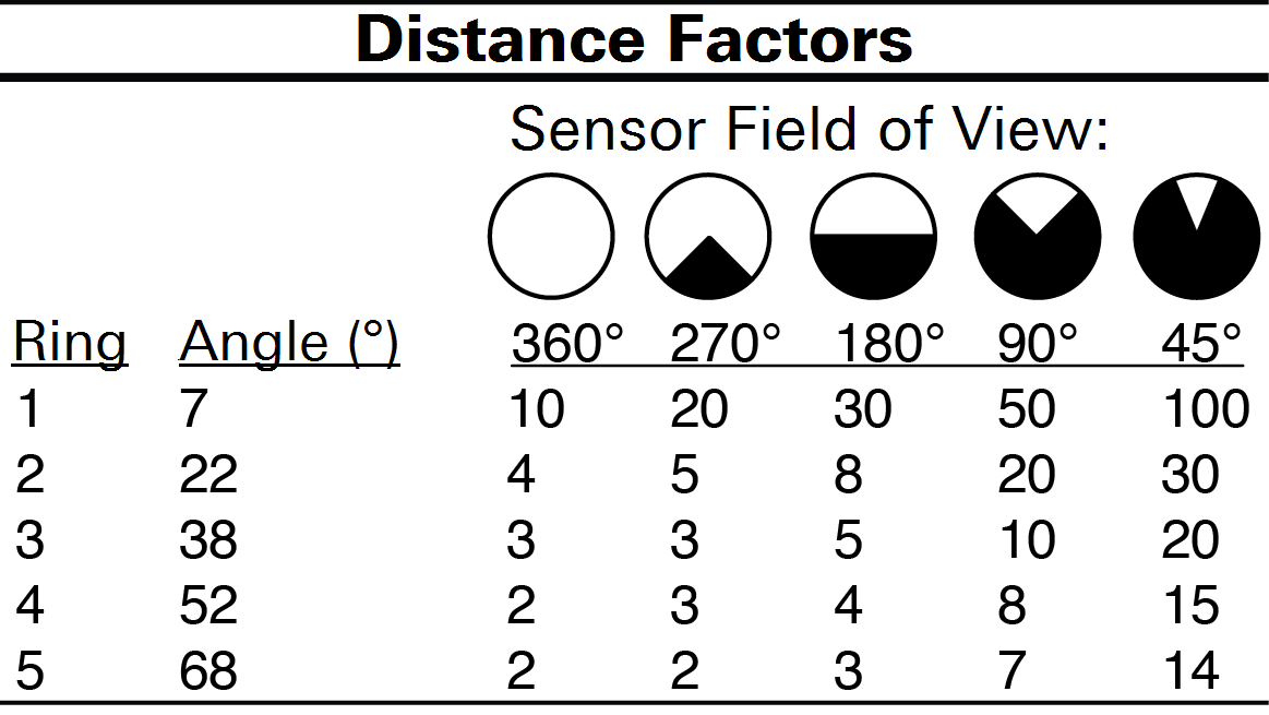
Table 4-2 provides guidelines for determining the minimum distance from the sensor as a function of foliage element size and zenith angle. To determine how close a particular leaf size can be to the sensor, find the column for the view cap being used in Table D‑2. Divide the values by the number of B readings to be made and multiply the results by the leaf width (cm).
|
The formula for determining whether a leaf is too close to the sensor is:
D‑2

where d is the distance factor from Table D‑2, B is the number of B readings, and w is the leaf width (cm).
For example, with no view cap and only one B reading, a 5 cm leaf should be 50 cm ((10/1)×5) away at 7°, 20 cm ((4/1)×5) away at 22°, and 10 cm ((2/1)×5) away at 68°.
Derivation of equation 4-2
One of the LAI-2200C assumptions (Assumptions) is that the foliage elements are small compared to the sensor field of view. Lang and Xiang (1986) derived a formula for the error as a function of foliage area and sample area: If R is the ratio of sample area (the region over which gap frequency determinations are made) to the area of an individual leaf, then the factor (E) by which the gap frequency is in error is
D‑3

We apply this analysis to an LAI‑2250 sensor by considering the sample “area” to be the distance around a particular ring’s view at a distance from the sensor that corresponds to the closest foliage. For example, the view of ring #2 is centered at 22°. If the closest foliage at 22° is 50 cm from the sensor, then the sample size for that ring (assuming the full 360° view) is (2π)50(sin(22))=118cm. If the leaf width is 5 cm, then R in equation 4-3 is 118/5 = 24, and the error is 1.02 or 2%.
Table D‑2 (Distance Factors) is for an error (E) less than 5%, requiring the ratio of view circumference to leaf width (R in equation 4-3) to be at least 10.6.