Tour #6: Configuration Introduction
OPEN can be configured to do many things (e.g. use a light source, do soil respiration, etc.). This tour will acquaint you with some basic concepts about managing configurations in OPEN. If you’d like more details on configurations, see Chapter 16 in the instruction manual.
Configuration Basics
We will start with the factory default configuration, make some changes, and see how to track and store them.
Experiment #1 Making Configuration Changes
- Start with Factory Default
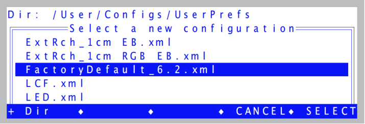
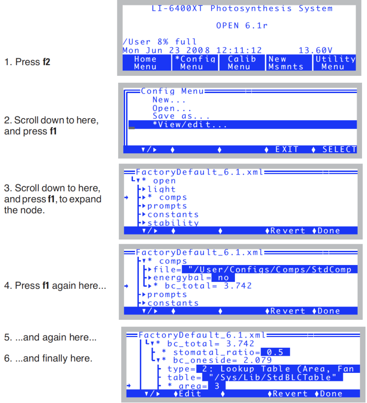
- To implement this, go to the Config Menu and select “Open...”. If asked to select a configuration (this happens if there is more than one file in the list) (Figure 3‑97), select “
FactoryDefault_6.2.xml”. - View the Configuration Tree
- Select the bottom item, “
View/edit...”. This will show you all the settings in the current configuration. You will be looking at a tree (Figure 3‑98). f1 will open and close nodes in the tree. - Now, let’s make some changes to the configuration and see what happens.
- Change leaf area
- Press escape a couple of times to get to OPEN’s main screen, then enter New Measurements mode. Press the AREA = key (f1 level 3), and enter 3 for the leaf area.
- Change stomatal ratio
- Press the STOMRT= key (f2 level 3), and enter 0.5 for the new value.
- Return to OPEN’s Main Screen
- Press escape to leave New Measurements mode. There will be a message waiting for you in the form of an asterisk in the Config Menu key label (Figure 3‑99).

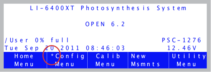
This asterisk alerts you to the fact that your configuration has been changed and not saved. To save a configuration, simply select Save as... from the Config Menu.
Rather than doing that quite yet, however, continue reading, and we’ll see something interesting about the Configuration Tree.
Experiment #2 Using the Configuration Tree
- Track the changes
- Tracking what changed is a matter of following the trail of asterisks1. Start by pressing f2 to get to the Config menu (Figure 3‑100).
- In the tree view, changed nodes (changed from how the config was stored) are shown with an asterisk. Also, any node that contains changed subnodes is shown with an asterisk. Thus, you can track down the specifics that have changed. In this example, the changed area and stomatal ratio nodes are at the end of the trail, as we would have expected.
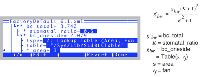
- Let’s look closer at the tree view, because the structure here tells us something. The total boundary layer conductance (bc_total) is computed from stomatal_ratio and a one sided value boundary layer value (bc_oneside). The one sided value, in turn, comes from a lookup table, leaf area, and fan speed (fan speed - fan - is just below area - you can scroll down and see it).
- Change area again from here
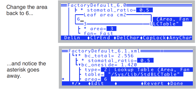
- Put the cursor on the area node, and press f2 (edit). Notice that you can change area (and a lot more) from here - you needn’t go to New Measurements mode to do so.
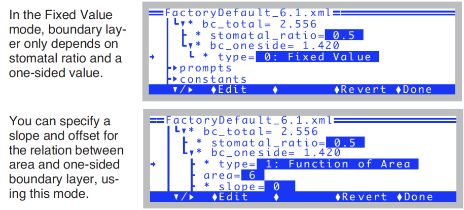
- The asterisk on area goes away because area has returned to is original (saved) state. Notice too that the value of bc_oneside has changed from 2.079 to 1.420. And, this changed the total boundary layer value (bc_total) from 2.742 to 2.556.
- Experiment
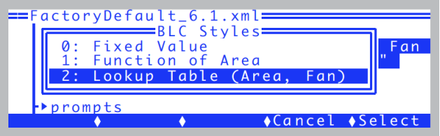
- Try out different leaf areas, and fan speeds by changing them from right here in the tree view using the Edit key (f2), and see the effect on boundary layer. Also, try out the type node, which determines how boundary layer is computed.
- You will notice that the tree changes structure a bit depending on how type is set. The other two (type 0 and 1) are shown below:
- Revert Everything
- Notice the f4 key (revert). With the cursor on a *-ed node, press f4. and you will be given a choice (Figure 3‑102) of revert all nodes back to the original state by pressing A, or just the current node by pressing T.
-
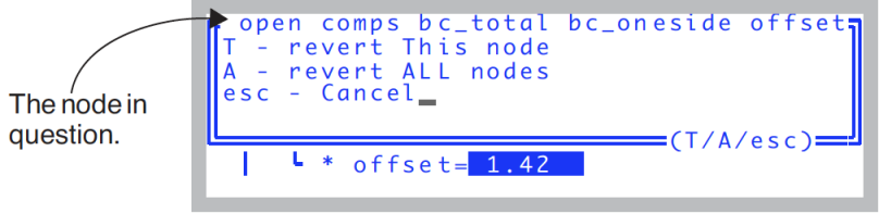
Figure 3‑102. Reverting one or more nodes.
Adding Prompts
Suppose you wish to make survey measurements, where each observation you log is on a different leaf, with a potentially different leaf area. Also, you’d like to add a column to the data that contains some identifier of that leaf, such as "Plot#". Finally, you wish to be prompted for leaf area and this identifier automatically each time you log a data record.
Experiment #3 Add Prompts for Plot# and Leaf Area
We’ll start in Config Menu|View/edit.
- Access the Prompts Node
- Navigate to <open> <prompts> <items> (Figure 3‑103).
- Open the Prompts Editor
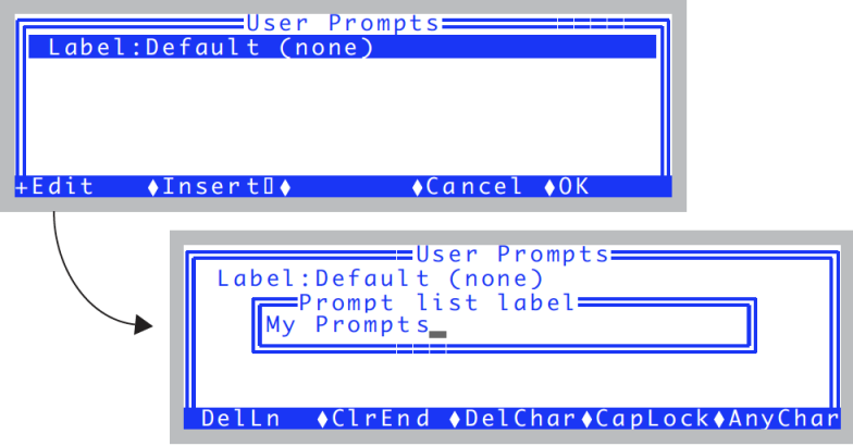
- With the cursor on the items node, press f2 (edit). You’ll see a label, and an empty list. Press f1 (edit), and name the list "My Prompts".
- Add Area to the list
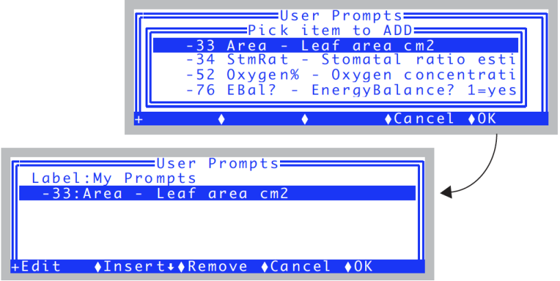
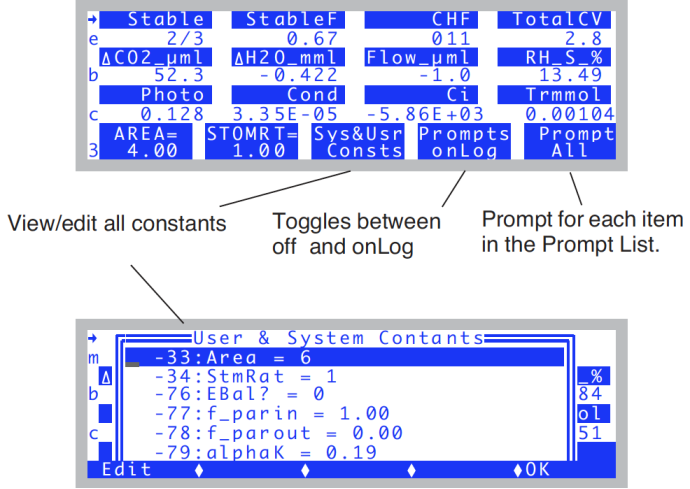
- Press f2 (Insert↓). You’ll be shown a list of constants. Find -33 Area, and press f5(ok) (Figure 3‑105).
- Add a user-definable system constant to the list
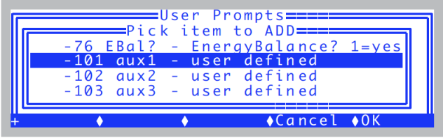
- There is no system constant named "Plot#", so we’ll create one, using one of the nine user-definable system constants. Press f2 (Insert↓) and scroll down to item -101 aux1, and press f5(ok) (Figure 3‑106).
- Change the label to "Plot#"
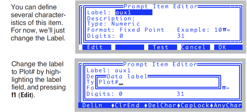
- You’ll be shown a dialog that lets you define some attributes of our system constant (Figure 3‑107). Make the label "Plot#".
- After you press f5(ok) to keep your change, the list should look like Figure 3‑108.
-
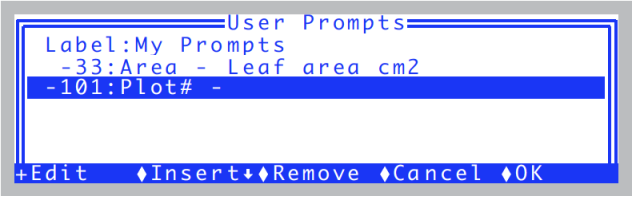
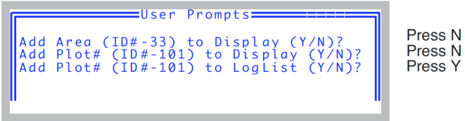
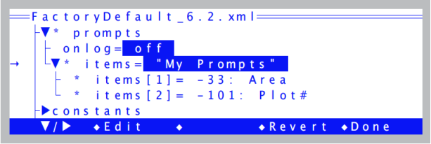
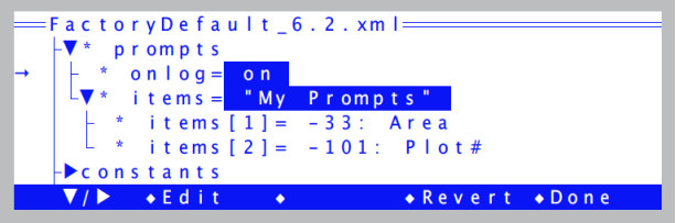
Figure 3‑108. Plot# added to the prompt list. - Exit the Prompt Editor
- Press f5(ok) to exit the prompt editor. You’ll be asked a series of questions about any items that you have added to the prompt list (Figure 3‑109).
- Once you are back in the View/edit screen, the items node should look like Figure 3‑110.
- Set for Automatically Prompting
- Move the cursor up to the
onlognode, and press f2 (edit) to change it from off to on (Figure 3‑111). - Try it out
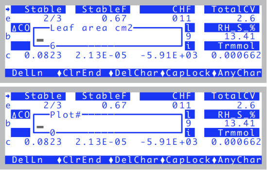
- Escape out of the Config Menu, go to New Measurements mode, open a log file, and log a record. You should be prompted for area and plot number (Figure 3‑112).
- Prompt Control in New Measurements
- Level 3 of the function keys have some prompt related items: f3, f4, and f5 (Figure 3‑113). Try out each one.
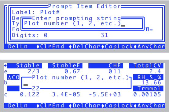
- The Prompting String
- One last detail: Back in Step 5, we left the description of our Plot# item blank. If you wish to have a more elaborate prompting sequence for a user constant, put it there. For example, if we go back into the configuration menu and change Plot#’s description as shown in Figure 3‑114, when it is prompted, that description is used, rather than the label.

Adding Computed Items
Suppose you wish to add an item that, unlike some constant like Plot#, needs to be computed. We illustrate that with a step-by-step example of adding a water use efficiency computation.
Experiment #4 Add Water Use Efficiency
First, we need a formula for water use efficiency. If photosynthetic rate is A (μmol m-2 s-1), and transpiration E (mol m-2 s-1), then water use efficiency W (in %) is
3‑1


(The 10-6 converts μmol to mol). So, what we need to add is something labelled WUE (for water use efficiency) that is computed from the quantities Photo and Trans that are already being computed. OPEN’s user-defined computations, like Photo and Trans, are defined in a ComputeList file (described in Chapter 15). One way to add WUE would be to change this file. OPEN gives us another method of adding user variables without actually touching the ComputeList file. Here’s how:
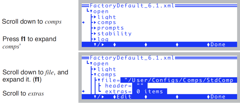
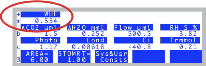
- Go to the extras node in the configuration tree
- Go to
Config Menu|View/edit. Navigate to <open> <comps> <file> < extras> (Figure 3‑115). - Add a new item.
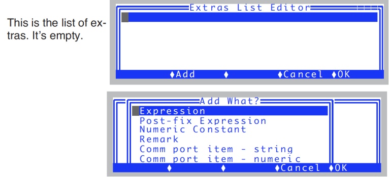
- With the cursor on the extras node, press f2 (edit), followed by f2 (Add) (Figure 3‑116).
- What we are adding is an expression, so highlight Expression, and press f5(ok).
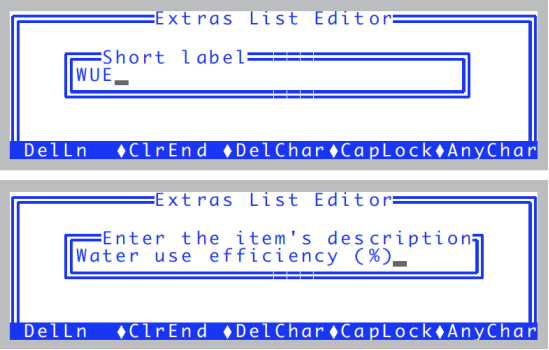
- Define the expression
- Enter the label and the description, as shown in Figure 3‑117.
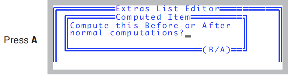
- Pick when it is to be computed
- With expressions, you can decide if they are to be computed before or after the normal user computations (items in the ComputeList). Since we are using items that are computed in the ComputeList (Photo and Trans), we want to compute WUE afterwards.
- Enter the equation
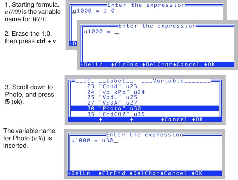
- The default formula for a new expression always starts out with our variable equaling 1.0 (Figure 3‑119). We need to edit this to implement the formula for WUE (equation (3-1) on page 3-84). To do this, a dialog known as the The Code Editor is employed, which is described in Editing Code on page 15-10 in the instruction manual.
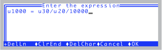
- Finish the expression (Figure 3‑120), either by using the ctrl+v method of inserting the variable name for transpiration in the right place, or by simply typing u20.
- When the equation is correctly entered, press f5(ok).
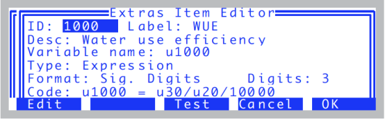
- Final details
- You’ll be presented with a dialog for this extra item (Figure 3‑121). Modify any of the fields you choose by highlighting the field, and pressing f1 (edit).
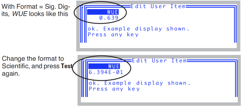
- Test it
- The test key (f3) will test the computation, and the display format (Figure 3‑122). This will allow you to experiment with various settings of Format and Digits, for example.
- Return to the List Editor
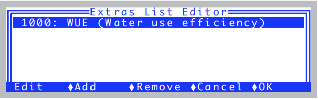
- Press f5(ok) to return to the List Editor (Figure 3‑123).
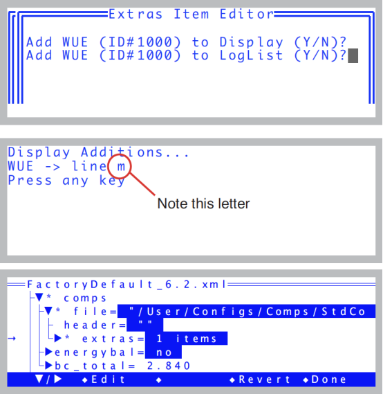
- Done Adding Extras
- Press f5(ok) to exit the List Editor. Because we have added something, we’ll be asked if we’d like to add it to the New Measurements display and the Log List (Figure 3‑124). Press Y for both.
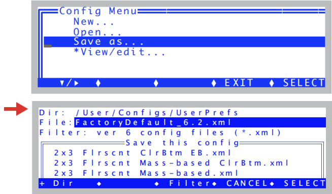
- Try it out.
- Go to New Measurements mode, and press m (or whatever line that was indicated back in Step 9) to see WUE (Figure 3‑125).
Saving Configuration Changes
You can save a configuration anytime by using the Save as... entry in the Config Menu.
Experiment #5 Saving your work
We’ll take a slow tour through what is normally a 1 or 2 step process, to point out some things that could be important to understand.
- Access the configuration save dialog
- It’s
Save as...in the Config Menu. - Note the directory: /User/Configs/UserPrefs
- Configuration files are all stored in the directory
/User/Configs/UserPrefs. These are the files that are shown when you are asked to pick a configuration, when you first run OPEN, or when you change to a previously stored configuration. - Note the filter: *.xml
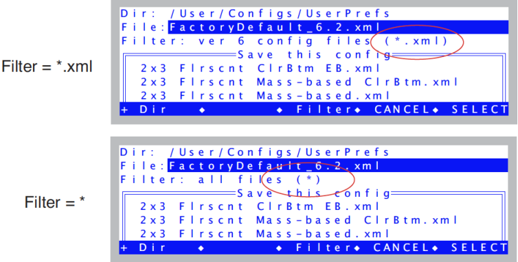
- There are two types of files in
/User/Configs/UserPrefs: those that end with ".xml", and those that don’t. There is a filter button (f3) that will toggle the filter setting between "*" (show all files) and "*.xml" (show only .xml files). Try it (Figure 3‑127). - *.xml files are version 6.1 configuration files. If there are other files in this directory, they are from earlier versions (like 6.0). They are compatible. However, when you save a configuration, it will be a .xml file, regardless of how the filter happens to be set (i.e., you cannot save a configuration in the old format).
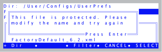
- Try overwriting FactoryDefault_6.2.xml
- Try saving the configuration over FactoryDefault_6.2.xml. It is a protected file, so won’t let you do it (Figure 3‑128).
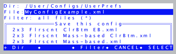
- Save it
- Make the name in the File box be what you want it to be, and press enter (Figure 3‑129). It doesn’t matter if you include the .xml or not. The file will get that extension regardless.
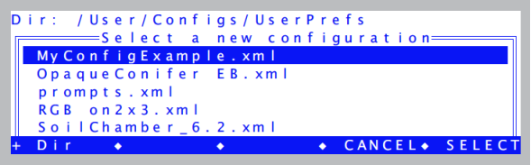
- The next time you are prompted to pick a configuration, the file you just created will be the default choice.
Congratulations - you made it through the end of the introductory tours. Chapter 4 builds on what you’ve learned here, and introduces you to proper measurement technique.