Example Background Programs
In this section, we present some examples that show how to carry out a measurement with a background program.
Early morning FoFm
Suppose you need to make a dark adapted fluorescence reading on a leaf the first thing in the morning, but don’t want to be there to do it. What you would rather do is start a BP the day before and put the instrument to sleep, leaving this BP running to do what needs to be done in the morning.
(A finished version of this program can be found in /home/licor/apps/examples/EarlyMorningFo.py). Specifically, we need the program to perform the following steps (each is followed by the actual BP step):
- Wait until 5 a.m. (WAIT).
- Get the instrument out of sleep mode (SETCONTROL).
- Wait a few minutes to let things warm up (WAIT).
- Open a log file (LOG).
- Log, getting an FoFm (LOG).
- Close the file (LOG).
- Go back to sleep (SETCONTROL).
To assemble this BP, do the following:
- Tap the Open/New tab, then New.
- This will take you to the Build tab, with an empty list.
- Insert a PROPERTIES.
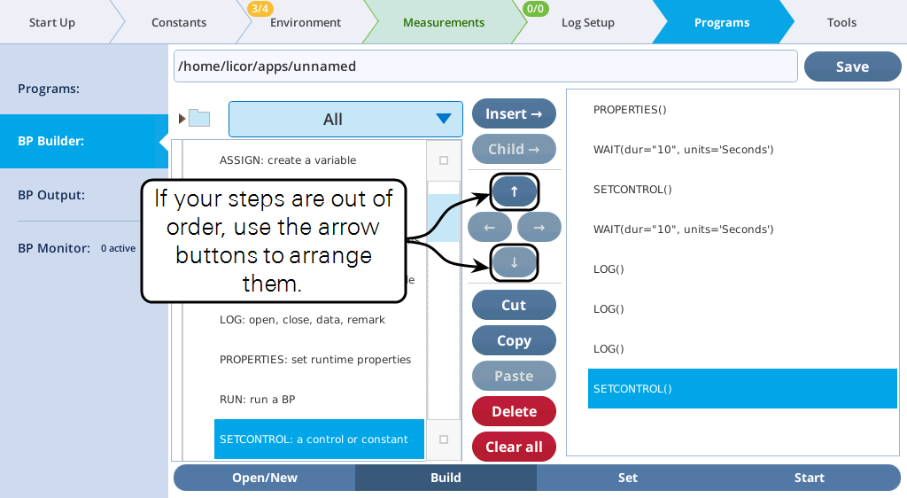
- Tap on PROPERTIES in the Steps section on the left, then tap Insert→.
- Insert a WAIT below it (with PROPERTIES highlighted on the right, and WAIT highlighted on the left, tap Insert→).
- This will become the item that waits until dawn.
- Continue, until the list looks as shown in Figure 13‑21.
- Tap on the Set tab, and configure each step according to Figure 13‑22.
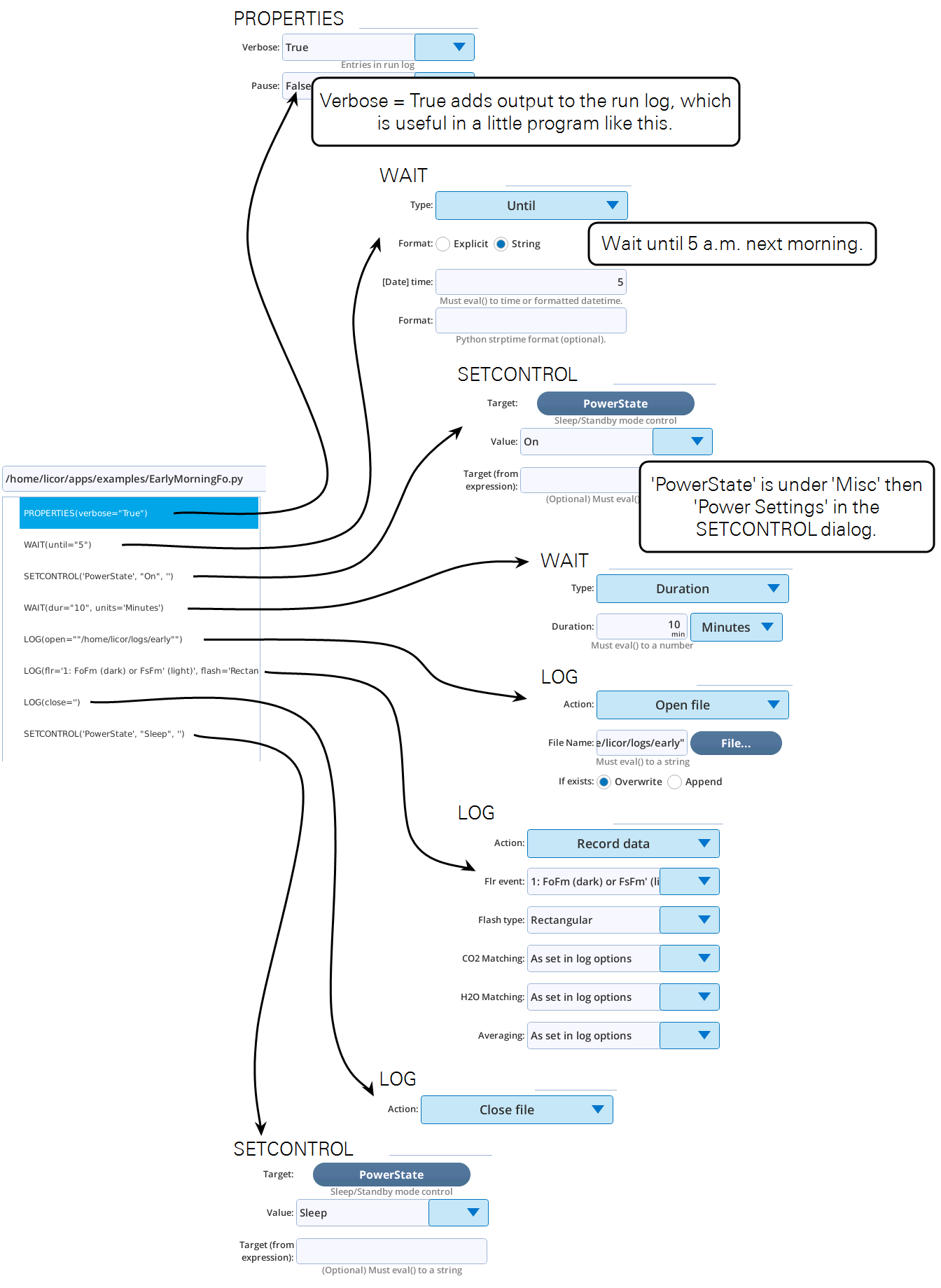
Note that we are doing three different things with LOG: open, write to, and close a file.
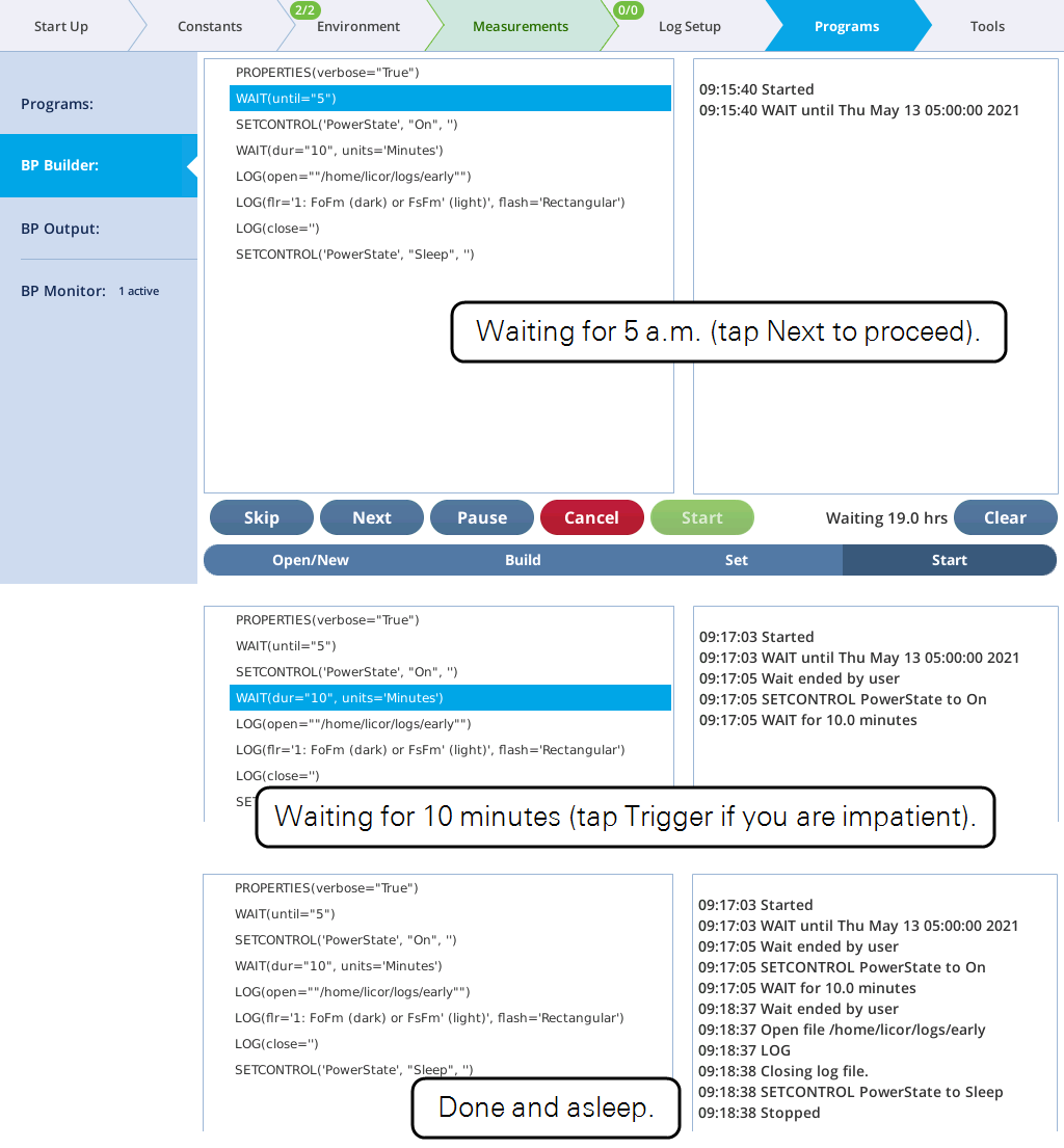
Test the program by tapping the Start tab, and then tap the Start button. Immediately we are waiting until 5:00 the next morning. Tap Trigger if you don’t want to wait that long.
Variations on AutoLog
Autologging (logging at regular intervals for some fixed amount of time) is very simple with a BP, but there are some useful variations on this theme that are good to know, including
- Log events can take variable amounts of time (matching, fluorometry, etc.), so how can we get precise log intervals?
- What if we want the log interval to change with time?
- What if we want to start or stop based on some environmental condition, rather than just the clock?
Timing
Let’s start with a basic autologging program (Figure 13‑24) which does a LOOP lasting 10 minutes (autolog duration) that contains a LOG and a WAIT (the logging interval).
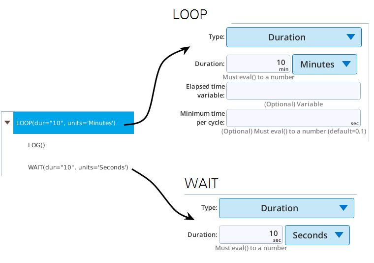
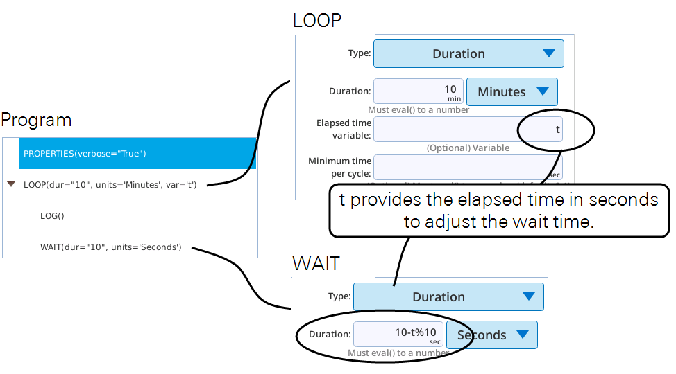
A potential shortcoming of this program is that it does not account for how long the LOG takes, which might range from about half a second to many seconds, depending on matching, fluorometer actions, and so on. If you were trying to log every 1 or 2 seconds, then this program would be a little frustrating because the log interval might often be longer than that. We could explicitly time the log in our program and adjust the wait time accordingly, but LOOP provides an easier way to accomplish that (Figure 13‑25).
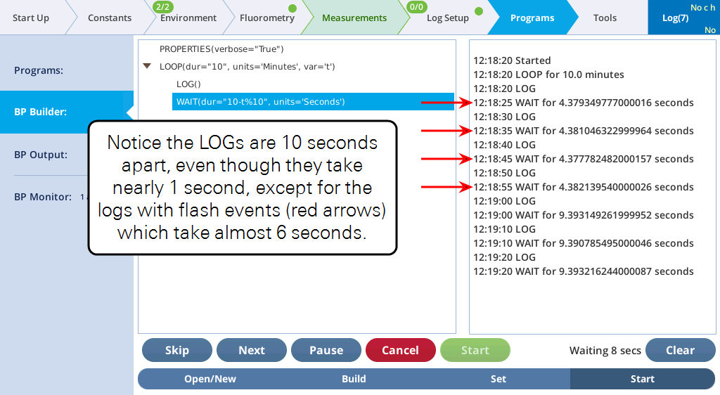
Let’s see this program in action. With a log file open, and a PROPERTIES statement added to get the actual time sent to the WAIT statements, we get Figure 13‑26.
There is yet a third method, and it is even easier (Figure 13‑27). LOOP (and WHILE) have a minimum time per cycle parameter that can be specified to regulate how often the loop repeats. At the end of the loop, it does an implicit wait if necessary to enforce that timing so we can get rid of our WAIT statement.
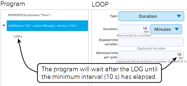
Another advantage of this last method is that both parameters for the autolog (duration and interval) are contained in the LOOP settings.
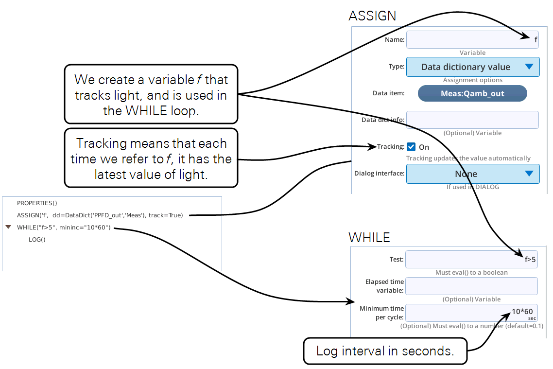
Log until sundown
Now that we know how to do an autolog program, let’s try another variation, this time adjusting the duration. Instead of a fixed time duration, let’s make it log until some environmental condition is met. Specifically, we’ll make a program to log a data record every 10 minutes from the time we start the program until the sun goes down. We’ll assume there is an external quantum sensor measuring light, and define sundown as when the PAR reading goes below 5 µmol m−2 s−1.
(A finished version of this program can be found in /home/licor/apps/examples/LogTilDark.py).
Now let’s test this program, making sure there is enough light on the external quantum sensor so it will act like daytime. To simulate sunset after a test loop or two, simply cover the sensor.
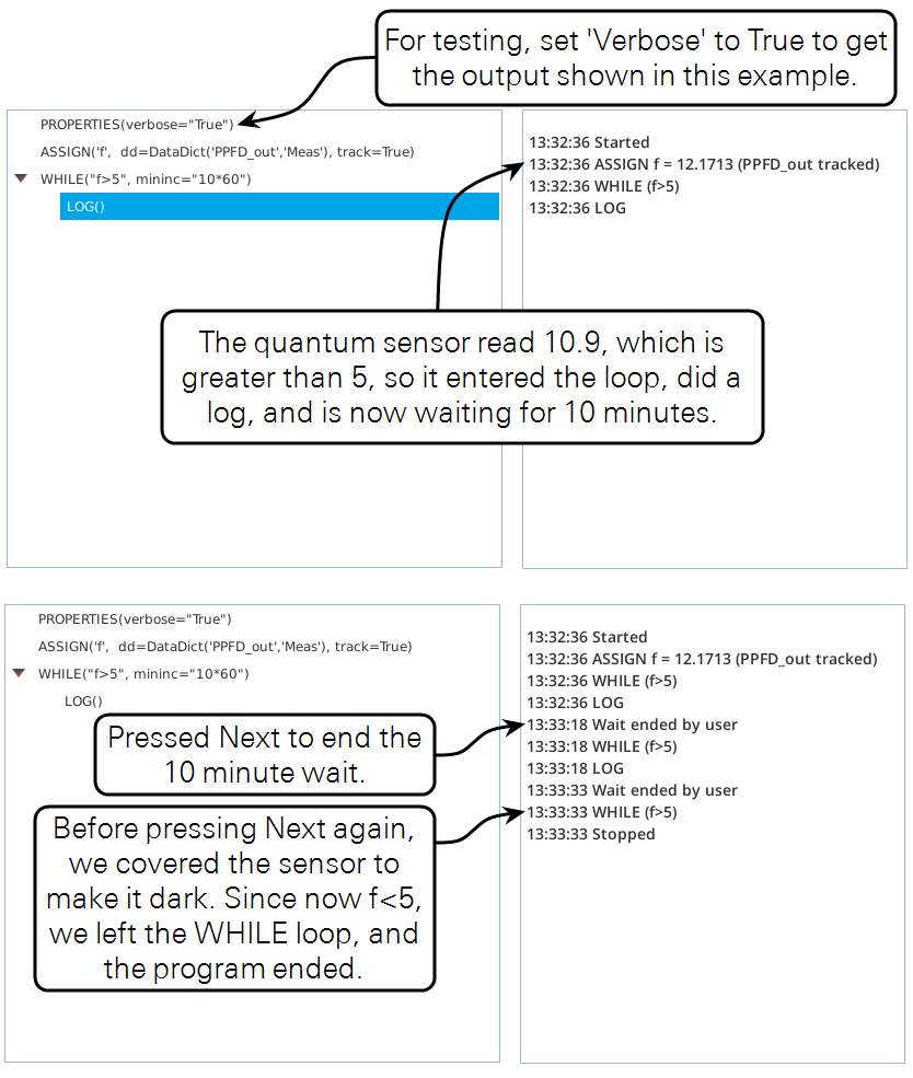
Running this program with Verbose=False (in the PROPERTIES step) will decrease the output to just the start and stop message, and the log events in between. This is how a repetitive program like this should normally be run.
Varying the log interval
When recording the response of a leaf to an abrupt environmental change (e.g., light level), there might be multiple time scales you want to capture, from the very rapid (photosynthesis) to the very slow (stomatal conductance). While one option might be to log as fast as possible for a long time, a more efficient method is to start logging frequently and slow down as time goes by.
BPs provide a couple of ways to do that.
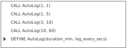
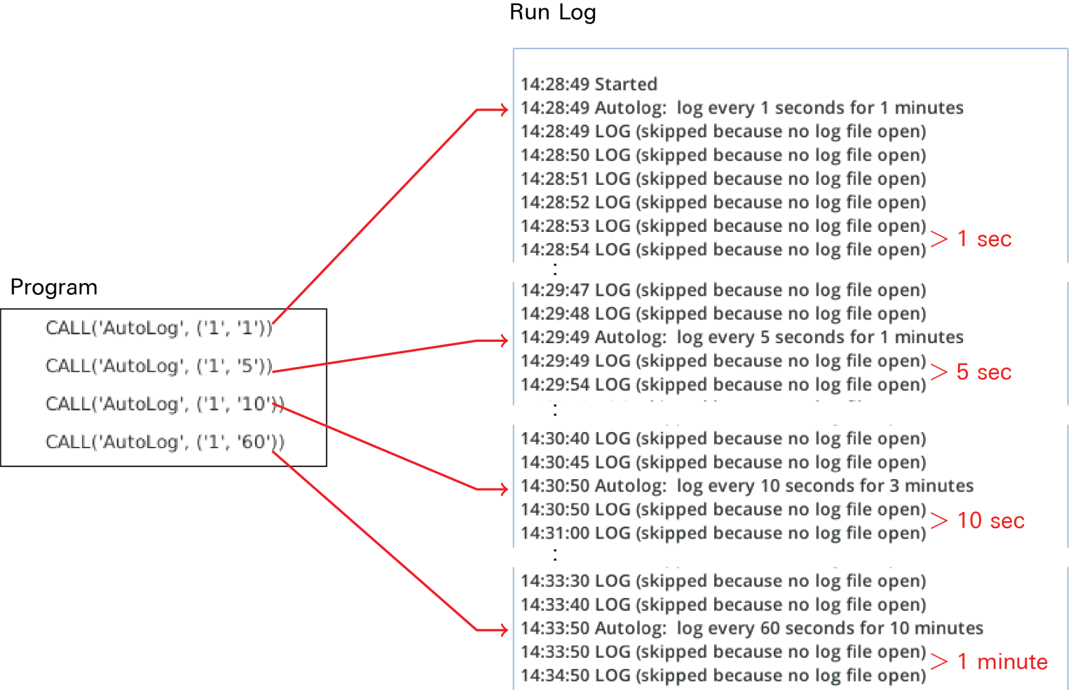
One method is to chain together a series of program loops, each with differing durations and wait intervals, such as log every 1 second for 1 minute, then every 5 seconds for 1 minute, then every 10 seconds for 3 minutes, then 60 seconds for 10 minutes.
Let’s assemble a BP that does this, and in the process learn something about BP functions (CALL and DEFINE):
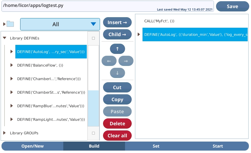
- Tap the Open/New tab, then New.
- This will take you to the Build Sequence tab, with an empty list.
- Add a CALL (With CALL highlighted on the left, and tap Insert→.)
- Add the function DEFINE AutoLog (With CALL highlighted on the right, scroll down to the Library DEFINEs section of the box on the left, tap on Define AutoLog, and tap Insert→.)
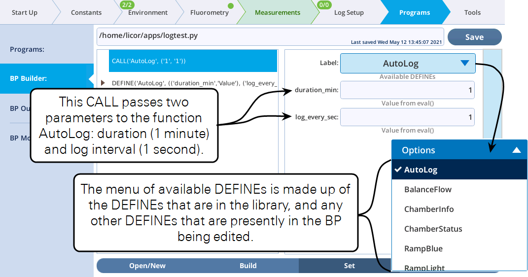
- Change to the Set screen, and configure the CALL to call the correct subroutine Figure 13‑31.
- Now change back to Build, highlight the CALL AutoLog on the right. Tap Copy, then, Paste, Paste, and Paste.
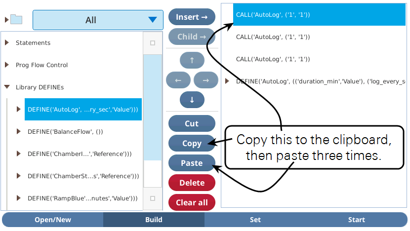
- Now change back to Set, and adjust the configurations on the three new AutoLog CALLs.
Up to now, we haven’t examined what a DEFINE looks like in a BP. Let’s do that now, and see what is inside the AutoLog DEFINE (Figure 13‑33).
The parameters for a DEFINE consist of a name, a parameter count, and names for each parameter. You can also specify if each parameter is passed in by value or reference (Step reference).
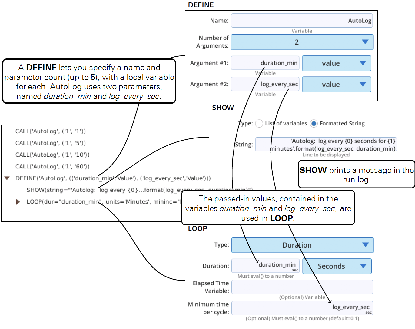
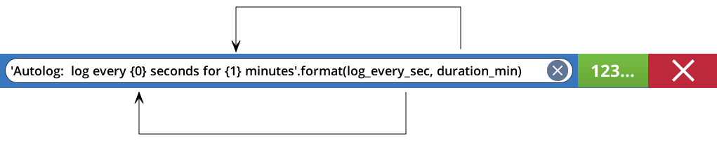
If you are wondering how the SHOW is printing the run log message you see in Figure 13‑34, it uses the built-in function format() for building a formatted string.
Because this AutoLog DEFINE is in the library, and we haven’t changed anything about the copy we added to our BP, we don’t really need it: We can delete it from our BP and the program will still work just fine.
There is another approach to varying log intervals after an event: make a function that provides the log interval as a function of time after an event. Lets say we want a logging interval that looks something like Figure 13‑35, which would be provided by a logistical expression such as
13‑1

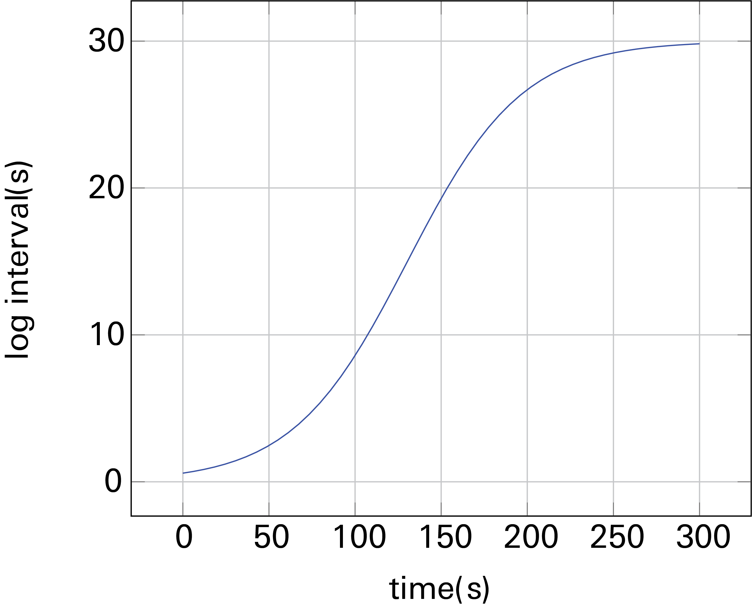
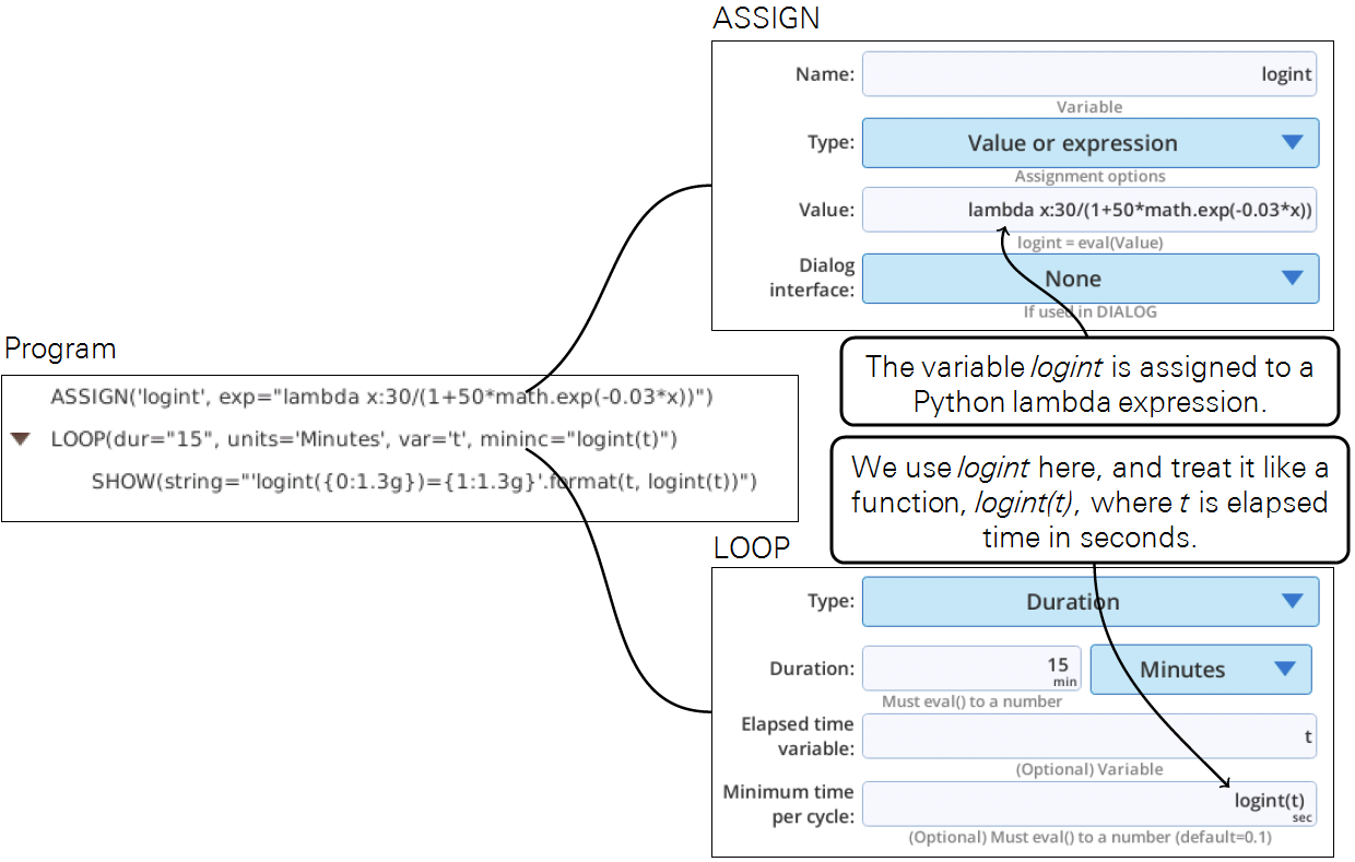
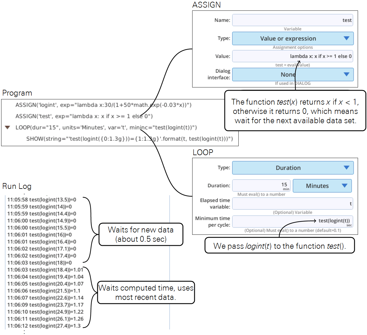
Implementing a function like this is very easy in a BP (Figure 13‑36). Creating a simple function is just like assigning a variable, but by preceding the definition with lambda x: (this is a Python construct), we declare logint to be a single parameter function, with x as the independent variable. The only thing in the loop is a SHOW statement to print out elapsed time and the computed loop trigger interval (formatted to show 3 significant digits).
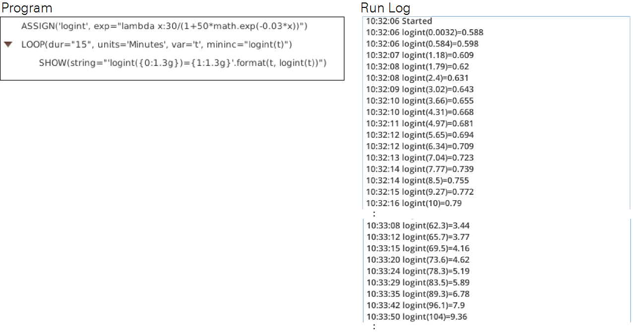
When run, this program produces the output as in Figure 13‑37. The loop starts out running about every 0.5 s, and increases from there.
At this point, we need to interject a bit of reality: the LI-6800 gets new data sets at 2 Hz, so it makes no sense trying to log any faster, and even if you could, you probably do not want to log two identical records. What we need, when we are logging rapidly, is a way to synchronize the log interval to when data is available.
Fortunately, there is a way to do that, and that is to set the ‘minimum time per cycle’ parameter in a LOOP to 0. Then, instead of waiting for the clock to tell it when to launch another cycle, it waits for a new data set to be ready.
Let’s adapt the program to use 0 for any logint(t) that computes to less than 1 second (Figure 13‑27).
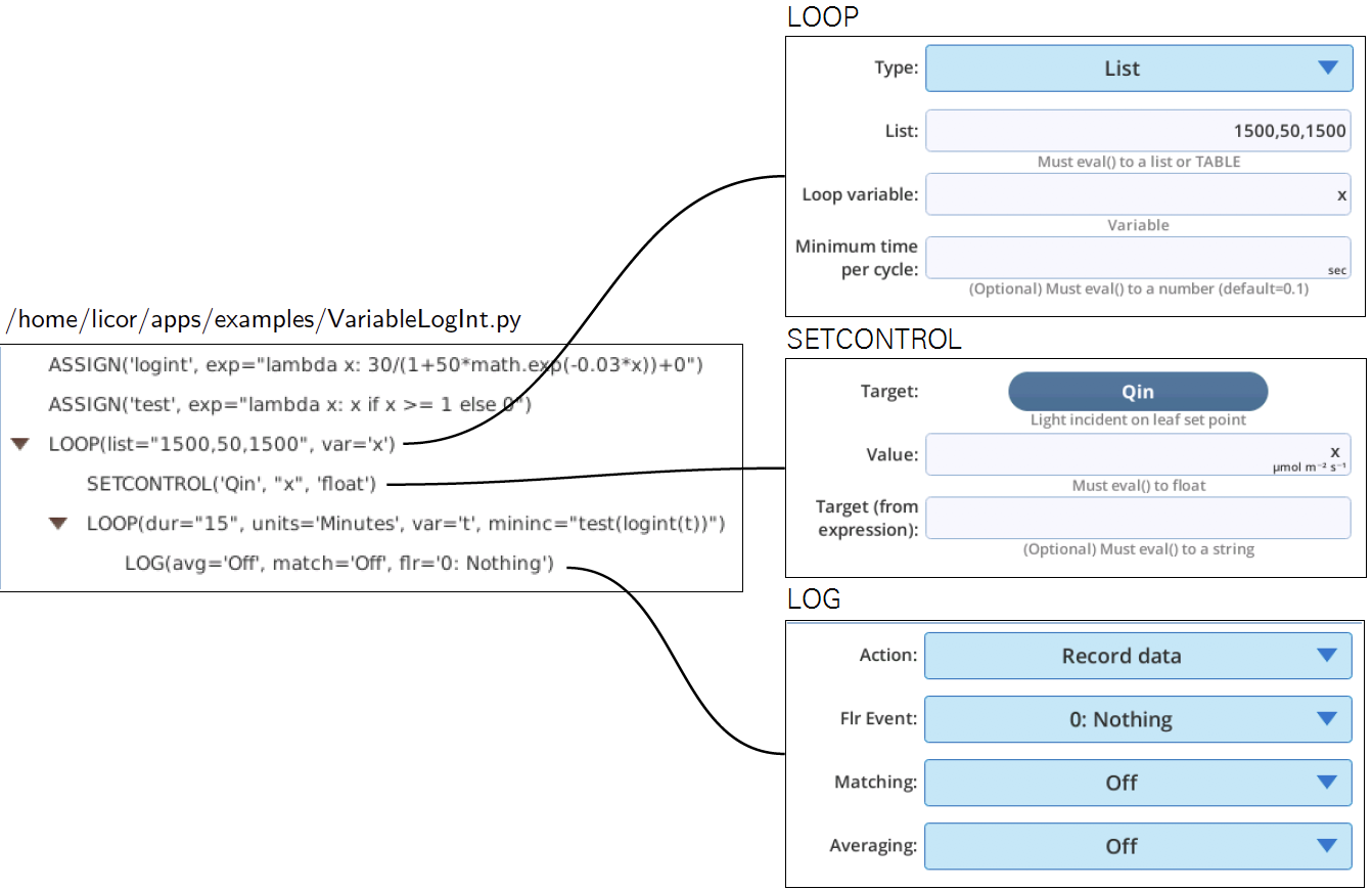
Let’s expand this program to do a couple of large step changes in light, and track the response with this timing function. The program is illustrated in Figure 13‑39, and is available at /home/licor/apps/examples/VariableLogInt.py.
Monitoring match mode
Suppose you are measuring isotopes in the air stream that is coming from the sample cell gas analyzer. You will need to know when the system is in match mode to know when to ignore that measurement (match mode puts reference air to both cells). A simple BP can monitor the system, and set a spare DAC channel to signal when match mode is active.


/home/licor/apps/utilities/MatchWatcher.py.Record and replay a time series
This example has two parts. In Part 1, the objective is to record a time series of light intensity to a file. This would be useful, for example, in an understory with passing sunflecks. In Part 2, use that file to drive a light source through the same time series of light intensities.
For the data recording part, we won’t use normal logging, as we just need a time stamp and light sensor value. A BP can do this for us easily, and Figure 13‑42 illustrates a test version, since it outputs to the run log, and only runs for 10 seconds.
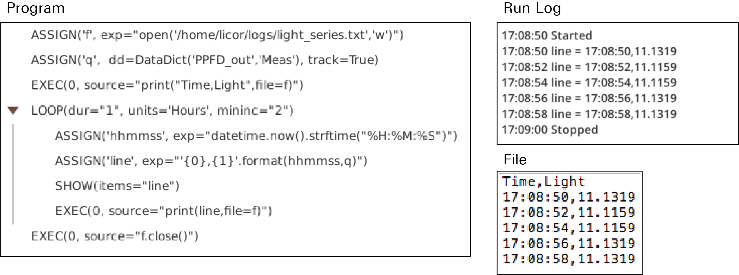
A discussion of the program steps follows:
- Use ASSIGN to open a file (using the Python expression for this), assigning f to the file object.
- Use ASSIGN to track the external quantum sensor with a variable named q.
- Write a header (“Time,Light”) to the file using a Python print statement inside of an EXEC step. Note the reference to the file (file=f) in the print.
- Use ASSIGN to make a variable hhmmss that captures current time in hh:mm:ss format. (The Python datetime module is available and is used for this.
- Use ASSIGN to build the observation line for the file, held in variable line.
- Use SHOW puts the line in the run log. (Strictly for debugging - we’ll get rid of this in the final version.)
- Write the line to the file using
print(), putting it all in an EXEC statement. - When the loop is done, close the file with
f.close(), inside an EXEC.
The real version of this program is in /home/licor/apps/examples/GetTimeSeries.py, minus the SHOW statement, and set to run for 1 hour.
Variations. For higher speed data, set the system averaging time to 0 (add a SETCONTROL before the LOOP, and target it to SysConst:AvgTime, which you’ll find under Constants, then System in the Control Dictionary), and make the time/cycle in the LOOP equal to 0 (this triggers the cycle each time new data is ready.)
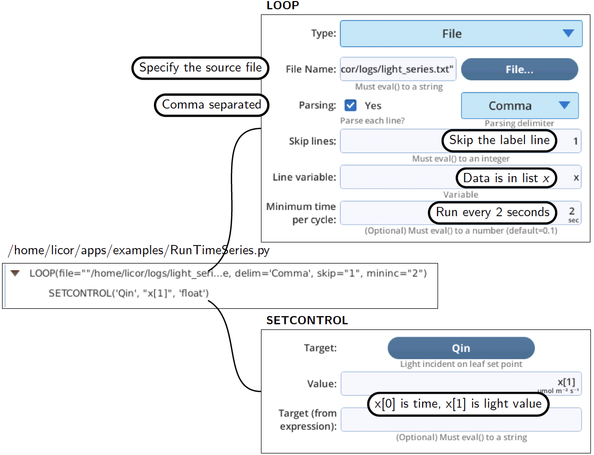
Part 2 is making a BP to use this file. All that is required is 2 steps (Figure 13‑43). The program is also available on /home/licor/apps/examples/RunTimeSeries.py.
Question: How would you modify this program to log the leaf response while it replays the time series?
The answer: don’t even try. Instead, run this program to drive the light source, and use a separate, concurrent autologging program (BP or conventional Program) to do the logging. Trying to do both is easy with separate programs, but combining them into one is more difficult. This is the power of BPs - you can split complicated tasks into simple, independent pieces.
Variations on that theme: You could launch both the autolog and the light control programs from a third BP (use the RUN keyword and the program’s file name), or you could launch the autolog BP from the light control BP, or vice versa.
Those are exercises left to the reader.