Custom events

LI-6800 Software version 2.1 (and fluorometer/head firmware version 1.4.21 and higher) supports a user-defined custom flash. With this new feature, the user can define up to 38 steps to be executed during a flash, and in each step specify duration, modulation rate, output rate, intensities of red, blue far red, modulation beam peak intensity, and rate of change of red actinic intensity. We’ve used the term “flash”, but more generally this is an event, since it could be a dark pulse, or flash and a dark pulse, or anything combination of things you’d care to define.

There are two parts of a Custom event definition:

1. What happens during the event. This is determined by a series of steps that specify settings and durations. These steps can be viewed or edited in a table (The table editor).
2. The results and computations that are to be extracted from the event data. This is controlled by a list of commands that you specify (Meta commands).

Custom flashes are configured from the Fluorometry > Settings > Custom screen. A tour, with an example of how to use this screen, follows next.

A quick tour

For this tour, we’ll make a custom flash that will duplicate the action of a currently defined standard flash, in this case, an MPF. Then we’ll add on a dark pulse, making a combination MPF plus dark pulse in one event.

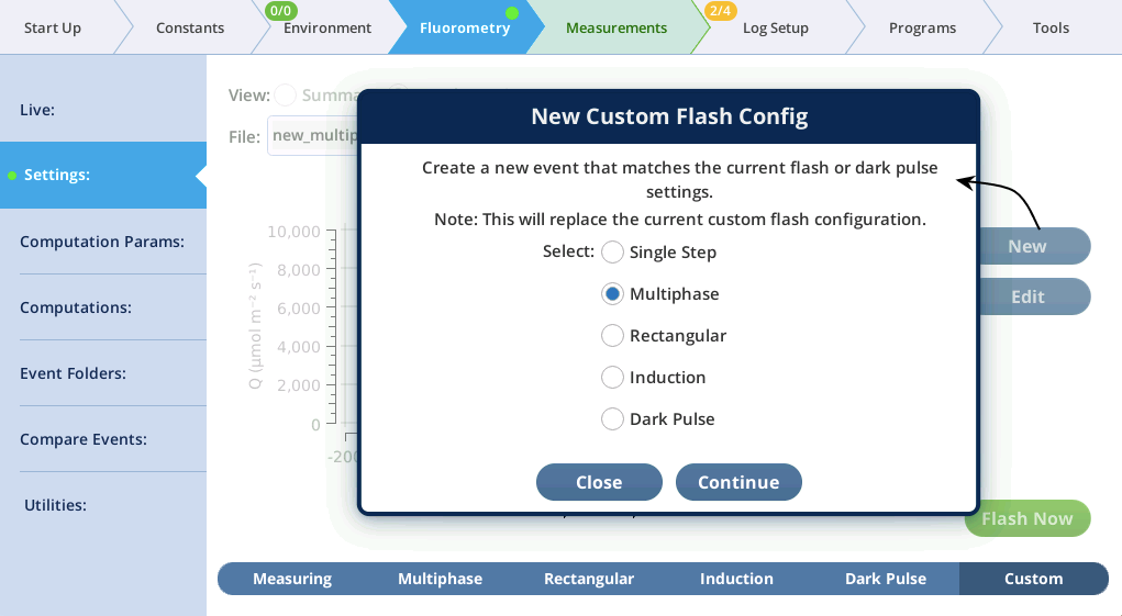
1. In the Settings > Custom screen, tap New, pick Multiphase, and tap Continue (Figure 8‑47).



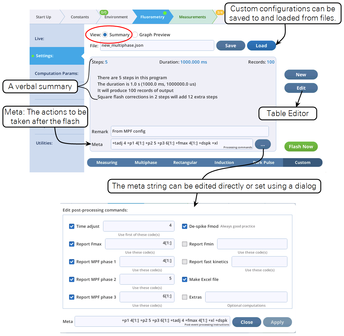
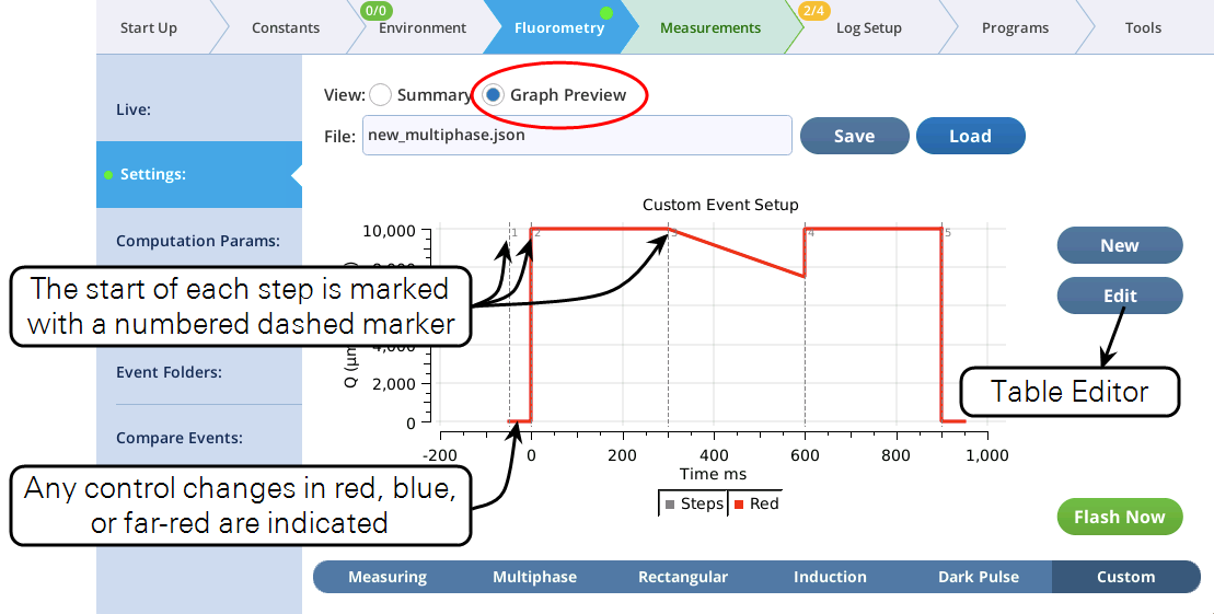
2. The Settings > Custom screen provides three views of the custom flash: text summary (Figure 8‑48), a graphical preview (Figure 8‑49), and an editable table (Figure 8‑50).







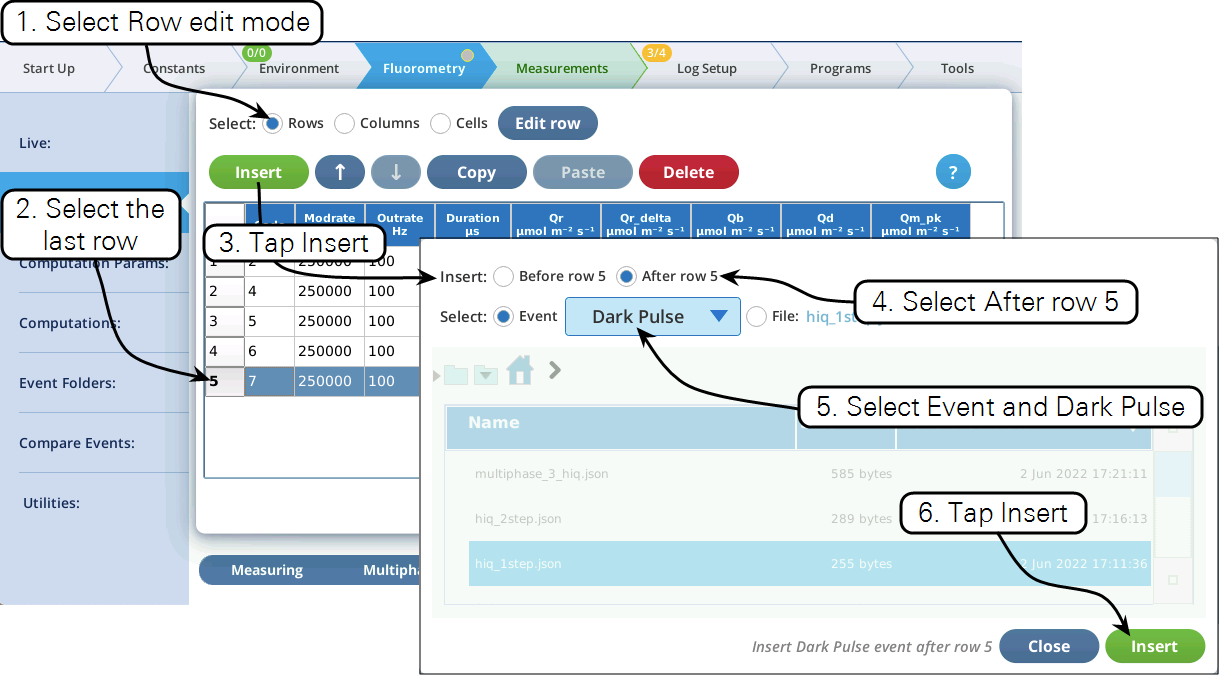
3. Now let's modify this event by adding a dark pulse to the end of it to measure Fo' all in one event. Go to the Table view, be sure you are in Row edit mode, tap row 5 to select it, then tap Insert (Figure 8‑51).



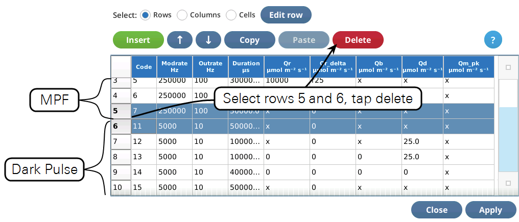
4. Once the two events are merged, we have to get rid of the final margin for the MPF (row 5, Code is 7), and the starting margin step for the Dark pulse (row 6, Code is 11). To do this, select them both (tap on row 5, drag down to row 6) and tap1 Note: we could also get rid of these two steps by setting the Duration value for rows 5 and 6 to 0, since 0 duration steps are simply skipped.Delete (Figure 8‑52). Then tap Apply to keep the changes you made.



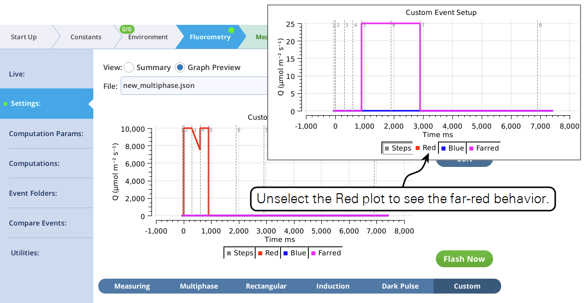
5. The graphical preview shows a combined MPF and dark pulse event (Figure 8‑53).



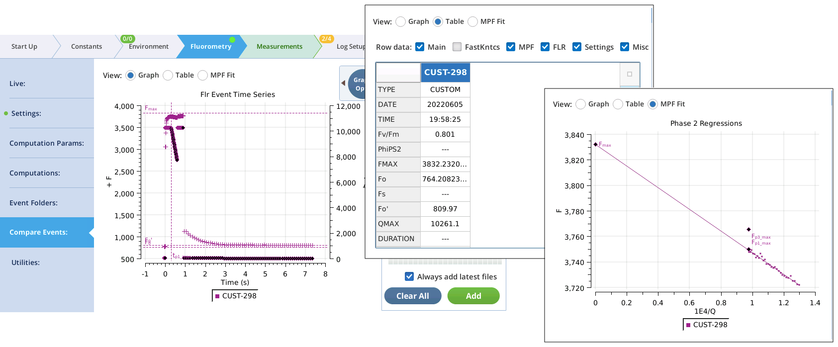
6. Test the custom event by tapping Flash Now , and examining the results in the Compare Events screen (Figure 8‑54).

Custom event definition files

Save and load

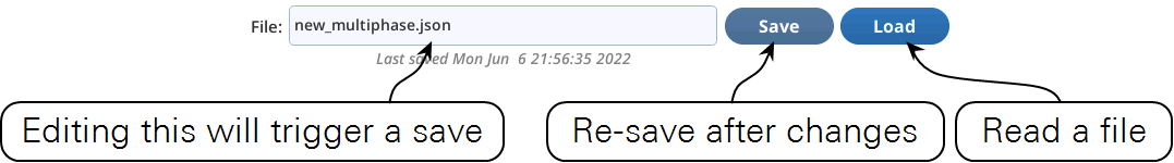
The Settings > Custom screen provides file access for saving and loading custom events (Figure 8‑55).

All files are saved in the directory /home/licor/flr/custom. You can create subdirectories simply by adding them to the name you enter. For example, if you enter

bob/test/sample.json

the directories bob and test will be created (if they don't already exist). Note that you are restricted to

/home/licor/flr/custom. If for example, you attempt to save to the logs directory, by entering

/home/licor/logs/sample.json

The resulting file will be

/home/licor/flr/custom/home/licor/logs/sample.json

The files are .json files. The .json suffix is automatically appended if you do not provide it.

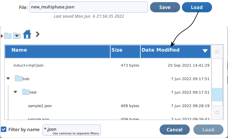
To read a saved file, tap Load. A file viewer dialog is provided for picking the file (Figure 8‑56).

File structure

The content of a custom event definition file is illustrated in Listing 8‑1. The structure is a map of strings. With the exception of the meta and remark items, each string contains space delimited values of the specified element for each step of the event. Note that some of the items, such as modrate, have only one value. The official number of steps is determined by the number of items in the duration string. When any another field is “short”, the last item in that string is assumed to apply at all remaining steps. (This particular example has not been through the Table Editor, which fills in all the missing values, so every item has the same number of steps.)

Listing 8‑1. A typical custom flash.py.

Archiving and backup

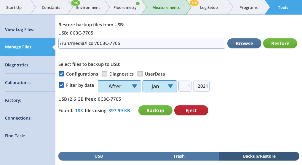
The /home/licor/flr directory is included as part of Configuration in the LI-6800s backup scheme (Figure 8‑57). The directory contains the custom folder (flash definitions), the extras folder (user defined meta computations), and the graphs folder (the Fluorometry > Compare Files graph saved settings).

Rules and Limits

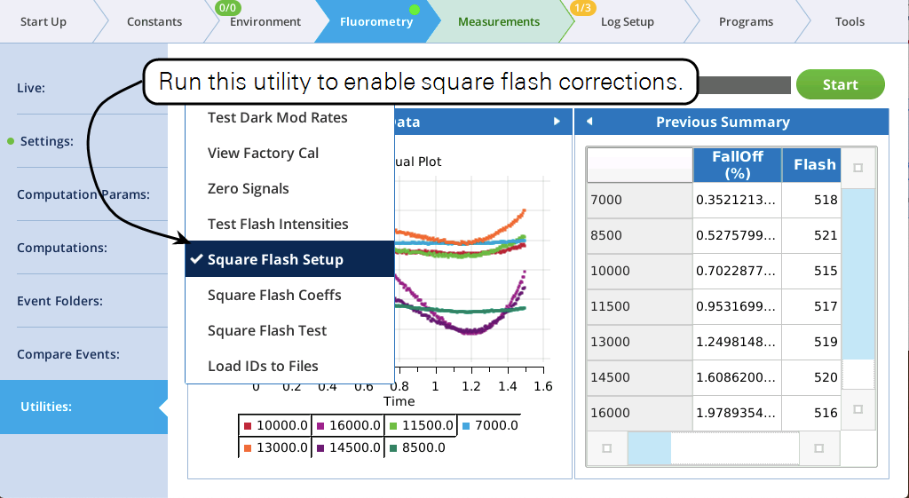
• Step limits. A custom flash can consist of no more than 38 steps (i.e., rows in the table). Square flash corrections (see Qr_delta) will reduce the available number of steps.
• Time limits. The sum of the Duration items can be no greater than 10 seconds. A single step's Duration has the same limit.
• Data limits. The total number of data records output for a flash cannot exceed 20,000. The number of output records n_i for the i^th step can be computed from.

8‑25

and the summation of output records over all N steps must satisfy

8‑26

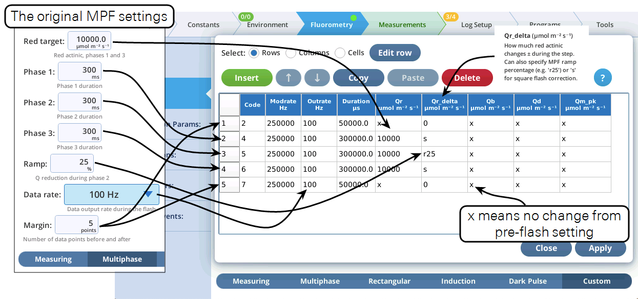
The table editor

Custom flashes are built and modified largely through the Table Editor (Figure 8‑58). The table’s columns represent the various things that you can specify about the fluorometer’s state, such as red actinic intensity, modulation rate, etc. Each row of the table represents a time step. In the example below, the 5 steps make up an MPF flash: step 1 is a pre-flash “margin”, steps 2, 3, and 4 are the MPF phases, and step 5 is a post flash “margin”.

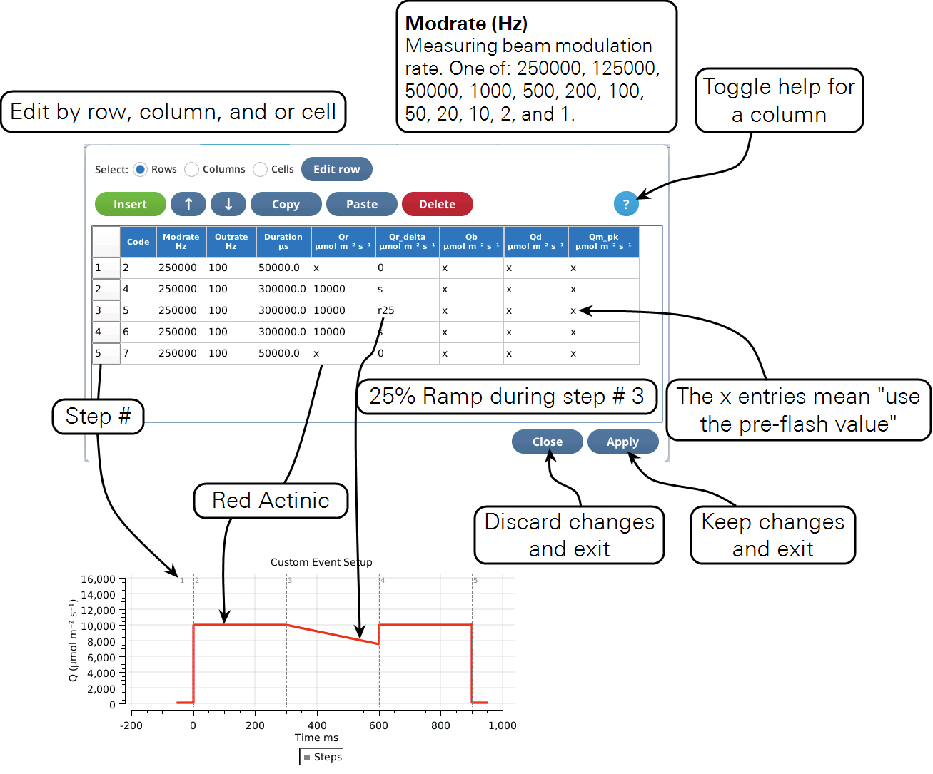
The table editor is a dialog; any changes you make are only retained if you tap Apply. To discard changes, tap Close.

Column help can be toggled on and off with the ? button.

Table 8‑10 provides a brief guide to each column in the Table view. For more details, see Custom event parameter reference.

Table 8‑10. Elements of a custom event step.

Label	Description	Entry Options	Units
Code	The step identifier number. All records output during this step will carry this identifier. Code numbers are closely associated with the meta string that specifies post-event processing options, described in Meta commands.	numeric (2 .. 53)
Modrate	Measuring beam modulation frequency.	numeric2 modrate can be one of: 250000, 125000, 50000, 20000, 10000, 5000, 2000, 1000, 500, 200, 100, 50, 20, 10, 5, 2, 1. If a different modulation rate is specified, the closest allowed value is used instead.	(Hz)
Outrate	Data record output frequency.	numeric3 outrate must be <= modrate, and evenly divisible into modrate. See Table 1‑8 on page 21 for examples. Nonconforming values are ignored, with the closest acceptable value used instead.	(Hz)
Duration	Duration of this step of the flash.	numeric4 Duration (µs) will be be an integer multiple of the output period (i.e. 106/outrate). Nonconforming values will cause the actual duration to be increased to the next allowable value. A value of 0 is acceptable, and causes that step to be skipped.	(µs)
Qr	The target intensity for the red actinic LEDs.	numeric	(µmol m-2 s-1)
	Set to percent of full scale	n%	(n in %)
	Use the pre-flash value.	x
Qr_delta	The amount to change (by linear ramp) the actinic LEDs during this step.	numeric	(µmol m-2 s-1)
	MPF ramp percentage. See equation 8‑27.	rn	(n in %)
	Square flash correction code. See Qr_delta.	s or sn	(n in ms)
Qb	The target intensity for the blue actinic LEDs.	numeric	(µmol m-2 s-1)
	Set to percent of full scale	n%	(n in %)
	Use the pre-flash value.	x
Qd	The target intensity for the farred LEDs.	numeric	(µmol m-2 s-1)
	Set to percent of full scale	n%	(n in %)
	Use the pre-flash value.	x
Qm_peak	The target intensity for the modulating LEDs.	numeric	(µmol m-2 s-1)
	Set to percent of full scale	n%	(n in %)
	Use the pre-flash value.	x

Basic controls

Three editing modes are available: Row, Column, and Cell.

Row editing

Row editing operates on selected row(s) of the table.

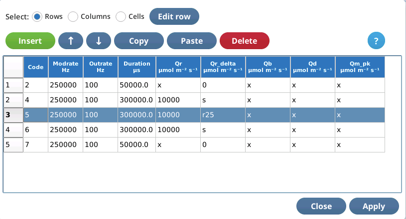
To select a row, simply tap it. Multiple selection is allowed.

To edit a selected row, tap Edit row. The edit string consists of space-delimited values corresponding to the 9 columns of the table.

Extra values are ignored. If you enter too few values, the "missing" ones remain unchanged.

Selected row(s) can be moved up or down with .

The table editor has a clipboard that can contain one or more rows. Selected rows are copied to the clipboard by Copy, and inserted into the table with Paste, which inserts the clipboard contents before the selected row. If no rows are selected, Paste becomes Append, which appends the clipboard contents to the end of the file. Note: the clipboard contents are maintained across "visits" to the table editor, allowing you to copy lines from one custom flash, and paste them into another.

Delete removes selected row(s) from the table.

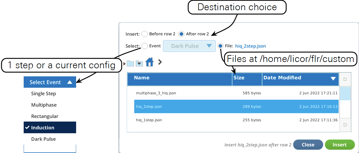
Insert allows external custom flash steps to be inserted into the table above or below the first selected row (Figure 8‑60).

Column Editing

Column editing operates the currently selected column. Tap in a column to select it.

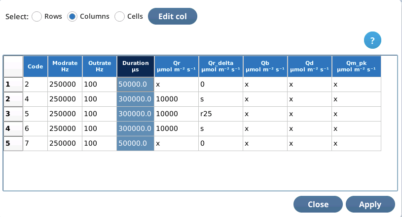
To edit the selected column, tap Edit col. The edit string consists of space-delimited values for that column for each row of the table.

If you enter too many entries, the extra ones are ignored. If you enter too few, the deficit is made up from the last value in the list. For example, to set an entire column to the same value, just enter one value when column editing.

Cell editing

Cell editing operates the currently selected cell. Tap in a cell to select it.

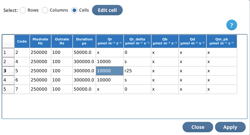
To edit a selected cell, tap Edit cell.

The Custom Flash Table Editor supports some special characters (see Table 8‑11) to make life easier when editing in Cell mode, depending on what column is being edited. For example, when changing the Qr value in the MPF flash table shown in Figure 8‑62, we really need to change Qr in steps 2, 3, and 4. This can be done with one cell edit by including a * with the new value (e.g., 15000*, or *15000, or 15*000 all do the same thing). Figure 8‑63. The * shortcut works for any column.

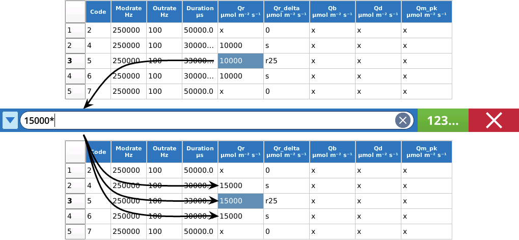
All of the cell edit helper characters are shown in Table 8‑11.

Table 8‑11. Editing shortcuts when in cell editing mode.

Cell	Char	Meaning	Example	Result
Duration	t	Value is total time (sum of previous steps) by the end of this step	650000t	Uses the preceding steps to computes the time (µs) it takes to make the total time 0.6s by the end of this step.
	ms	Value is in ms	50ms	50000
	s	Value is in s	1s	1000000
	p	Value is the number of points to log during this step	100p	Whatever duration (µs) it takes to log 100 points (based on Outrate for that step)
Outrate	p	Value is the number of points to log during this step	100p	Whatever output rate (Hz) it takes to log 100 points (based on Duration for that step)
Any	*	Change all like values in this column	15000*	All entries in this column that have this cell’s current value will be changed to 15000

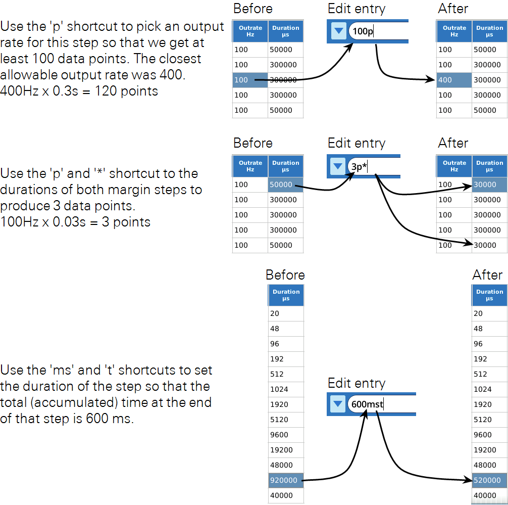
Some rules for using shortcuts:

• t can be used in combination with s or ms.
• p can not be used with s, ms, or t.
• * can be used in combination with any other shortcut character.
• Order or position do not matter. For example 100mst = t100ms = 10t0ms = 1ms0t0, etc.
• Entries with shortcut characters are not preserved - they are immediately converted to the units required by the column.

Figure 8‑64 presents some more examples.

Automatic rule enforcement

Several custom flash settings have a restricted range of possible values.

1. Code - Between 2 and 53
2. Modrate - One of 250000, 125000, 50000, 20000, 10000, 5000, 2000, 1000, 500, 200, 100, 50, 20, 105 5, 2, and 1 Hz are also legal, but not recommended..
3. Outrate - Depends on Modrate. Details in Outrate.
4. Duration - Will always be an even multiple of 10⁶/Outrate. Details are in Duration.

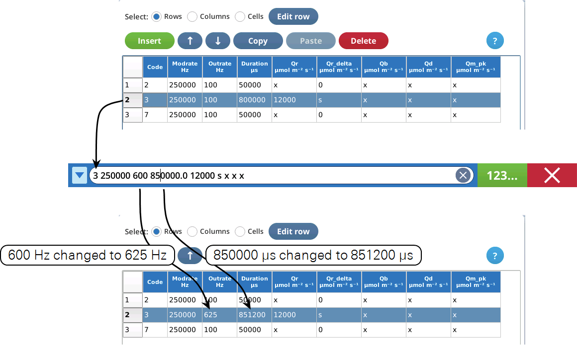
Please note that the fluorometer will quietly adjust any requested custom flash parameter to make it "legal" or workable, so entering an outrageous value for something will not hurt anything.

However, to make proper configuration more transparent, the Custom Flash Table editor will check each of your values as you enter them and adjust as necessary, so the values you see (after an edit) are the ones the fluorometer will actually use. This assistance occurs regardless of the edit mode (Cells, Rows, or Columns).

Custom event parameter reference

The columns in the Table editor represent the various degrees of freedom that you have to define a custom event. This section describes each.

Code

Code values are how steps are referenced for post event analysis.

Code values do not have to be unique. Rather, all steps that you might wish to include in a common analysis can contain the same code number. For example, the custom version of the induction flash has 11 code 3 steps. Here are the meta and code lines from Listing 8‑1:

Those 11 steps serve to smoothly adjust duration and output rates to provide high density output at the start of the flash, tapering off to less frequent output later on in the flash. The meta codes calling for finding the max value (+fmax 3) and the fast kinetic analysis (+fk 3) reference step 3, so all steps labeled 3 get included in those analyses. You could label them differently if you wish, but the meta codes would then have to reference a lot of code values, leaving you something like this

A step's Code value should be an integer between (and including) 2 and 53. The code values below 16 have always been used in standard ashes (RECT, MPF, INDUCTION, and DARKPULSE). Historically, the code value was used to trigger certain computations by the fluorometer itself. For example, if there were any steps with code 3, that would trigger an FMAX computation using all code 3 records. With custom event firmware, however, computations are only triggered via meta commands (see Meta commands), not code numbers.

Therefore, code numbers can be anything you want, between 2 and 53. They do need to be "in sync" with the meta commands, however.

Table 8‑12. Step codes and their historical meeting.

Code	Description
2	Pre-flash margin
3	RECT or INDUCTION flash
4	MPF Phase 1
5	MPF Phase 2
6	MPF Phase 3
7	Post-flash margin
8 - 10	unused
11	DARK pre margin
12	DARK part 1
13	DARK part 2
14	DARK part 3
15	DARK post margin
16 - 53	CUSTOM

Modrate

There are dependencies among modrate, outrate and duration. It all starts with modulation rate, which determines the basic time period (1/modrate) in which measurements and actions during the flash event occur. For a saturating flash, one normally uses the highest modulation rate (250 kHz), yielding a 4 µs event cycle period in which the fluorometer operates. See Figure 26 on page 47 for a detailed illustration.

Outrate

The outrate for a step, the frequency with which fluorometer outputs data, cannot exceed the modrate. Usually one uses a much lower outrate, providing averaging and a manageable data flow. However, outrate needs to divide evenly into modrate. Table 8‑13 shows the available outrate values for a few of the available modrate values.

Example: If moderate = 250000 Hz, the table indicates (by "ok") that 25000 Hz is an acceptable outrate (250000/25000 is an integer), but not 20000 Hz (250000/20000 is not an integer).

Table 8‑13. Allowable outrates and associated periods for 5 different modulation rates.

outrate	period	modrate (Hz)
(Hz)	(µs)	250000	125000	50000	20000	10000
250000	4	ok	—	—	—	—
125000	8	ok	ok	—	—	—
62500	16	ok	ok	—	—	—
50000	20	ok	—	ok	—	—
31250	32	ok	ok	—	—	—
25000	40	ok	ok	ok	—	—
20000	50	—	—	—	ok	—
15625	64	ok	ok	—	—	—
12500	80	ok	ok	ok	—	—
10000	100	ok	—	ok	ok	ok
6250	160	ok	ok	ok	—	—
5000	200	ok	ok	ok	ok	ok
4000	250	—	—	—	ok	—
3125	320	ok	ok	ok	—	—
2500	400	ok	ok	ok	ok	ok
2000	500	ok	—	ok	ok	ok
1250	800	ok	ok	ok	ok	ok
1000	1000	ok	ok	ok	ok	ok
800	1250	—	—	—	ok	—
625	1600	ok	ok	ok	ok	ok
500	2000	ok	ok	ok	ok	ok
400	2500	ok	—	ok	ok	ok
250	4000	ok	ok	ok	ok	ok
200	5000	ok	ok	ok	ok	ok
160	6250	—	—	—	ok	—
125	8000	ok	ok	ok	ok	ok
100	10000	ok	ok	ok	ok	ok
80	12500	ok	—	ok	ok	ok
50	20000	ok	ok	ok	ok	ok

Table 8‑14. Allowable outrates and associated periods for low different modulation rates, suitable for dark readings.

outrate	period	modrate (Hz)
(Hz)	(µs)	2000	1000	500	200	100	50	20	10
2000	500	ok	—	—	—	—	—	—	—
1000	1000	ok	ok	—	—	—	—	—	—
500	2000	ok	ok	ok	—	—	—	—	—
400	2500	ok	—	—	—	—	—	—	—
250	4000	ok	ok	ok	—	—	—	—	—
200	5000	ok	ok	—	ok	—	—	—	—
125	8000	ok	ok	ok	—	—	—	—	—
100	10000	ok	ok	ok	ok	ok	—	—	—
80	12500	ok	—	—	—	—	—	—	—
50	20000	ok	ok	ok	ok	ok	ok	—	—
40	25000	ok	ok	—	ok	—	—	—	—
25	40000	ok	ok	ok	ok	ok	ok	—	—
20	50000	ok	ok	ok	ok	ok	—	ok	—
16	62500	ok	—	—	—	—	—	—	—
10	100000	ok	ok	ok	ok	ok	ok	ok	ok
8	125000	ok	ok	—	ok	—	—	—	—
5	200000	ok	ok	ok	ok	ok	ok	ok	ok
4	250000	ok	ok	ok	ok	ok	—	ok	—
2	500000	ok	ok	ok	ok	ok	ok	ok	ok

Duration

The duration of a step is simply how long you wish the step to last, in µs. This is fairly simple, but there is a subtlety here, especially for short durations: the actual time a step lasts will always be an even multiple of the output period.

Suppose moderate = 250000 Hz and outrate = 25000 Hz. duration should then be a multiple of value in the period column in Table 8‑13, which is 40. Suppose we specified a duration of 500 µs. What happens? When that step executes, even though you asked for 500 µs, it will actually last 520 µs, since it needs to be an even multiple of 40. That extra 20 µs, however, is not long enough to average together enough points for the next output cycle, so those measurements go unused.

Qr

The Qr value determines the red actinic for the step. This is typically the primary item being changed for a flash. Square flash corrections and ramping can be done on this value, but those are controlled by the next item, Qr_delta.

Qr_delta

The Qr_delta element provides capabilities for ramping the red actinic during one step of a custom flash. For example, specifying a value of 100 will cause Qr to increase linearly during that step by 100 µmol m^-2 s^-1. A value of −1000 would cause it to decrease linearly by 1000 µmol m^-2 s^-1.

To specify a percent ramp (down) in the same way that an MPF phase 2 is done, use r followed (no space!) by an integer value that represents the percent ramp (e.g., r25). The fluorometer will compute the appropriate value of Qr_delta as

8‑27

where R is a percent ramp [0...100], and Qr0 is the value of red actinic prior to the flash.

The r code is useful when defining a flash step, because you might not know what Qr0 will be at the time of the flash’s execution.

Specifying a Qr_delta of s instead of a value will call for a square flash correction to be applied to that step. A square flash correction can be enabled for a maximum of 4 steps.

Also, square flash corrections count against the 38 total step limit. One square flash correction can add as many as 12 ”hidden” steps, depending on that step’s Duration. A square flash correction of a 1 second step uses 12 extra steps, but fewer if the step is less than 1 second. Table 8‑15 relates step duration (in ms) to the “cost” in steps of doing a square flash correction. For example, applying a square flash corrected to a step of 400 ms will reduce the total available steps by 7.

Table 8‑15. Cost of square flash correcting.

Duration (ms)	Steps
≤ 1,000+	12
≤861	11
≤733	10
≤615	9
≤506	8
≤408	7
≤320	6
≤241	5
≤173	4
≤115	3
≤67	2
≤28	1

Hint: Don’t “waste” a square flash correction on any step shorter than about 10 ms. Also, the correction is only applied if a square flash calibration has been done, and if the correction is enabled at the time of the flash.

Qb

Qb is the value of the blue actinic LEDs during a step. To leave these unchanged, simply specify a value of x.

Qd

Qd is the value of the far red LEDs during a step. To leave these unchanged, simply specify a value of x.

Qm_pk

Qm_peak is the value of the peak modulation for the red measuring LEDs. Since computations involving modulated fluorescence values in and out of an event need to be made using the same Qm_peak setting, this should normally always have a setting of x (no change).

Meta commands

The Meta specifier contains commands that tell the LI-6800 how to handle an event (flash or dark pulse), and what analysis computations to add to the event file, once the event data is received from the fluorometer. With standard events (RECT, MPF, INDUCTION, or DARK), the meta commands are automatic, and hidden. With a CUSTOM event, however, you have access to them to use as you wish.

Meta commands can be entered in the Meta field shown in Figure 8‑67. Note that a GUI is provided to assist with the commands. A summary of the meta commands is given in Table 8‑17.

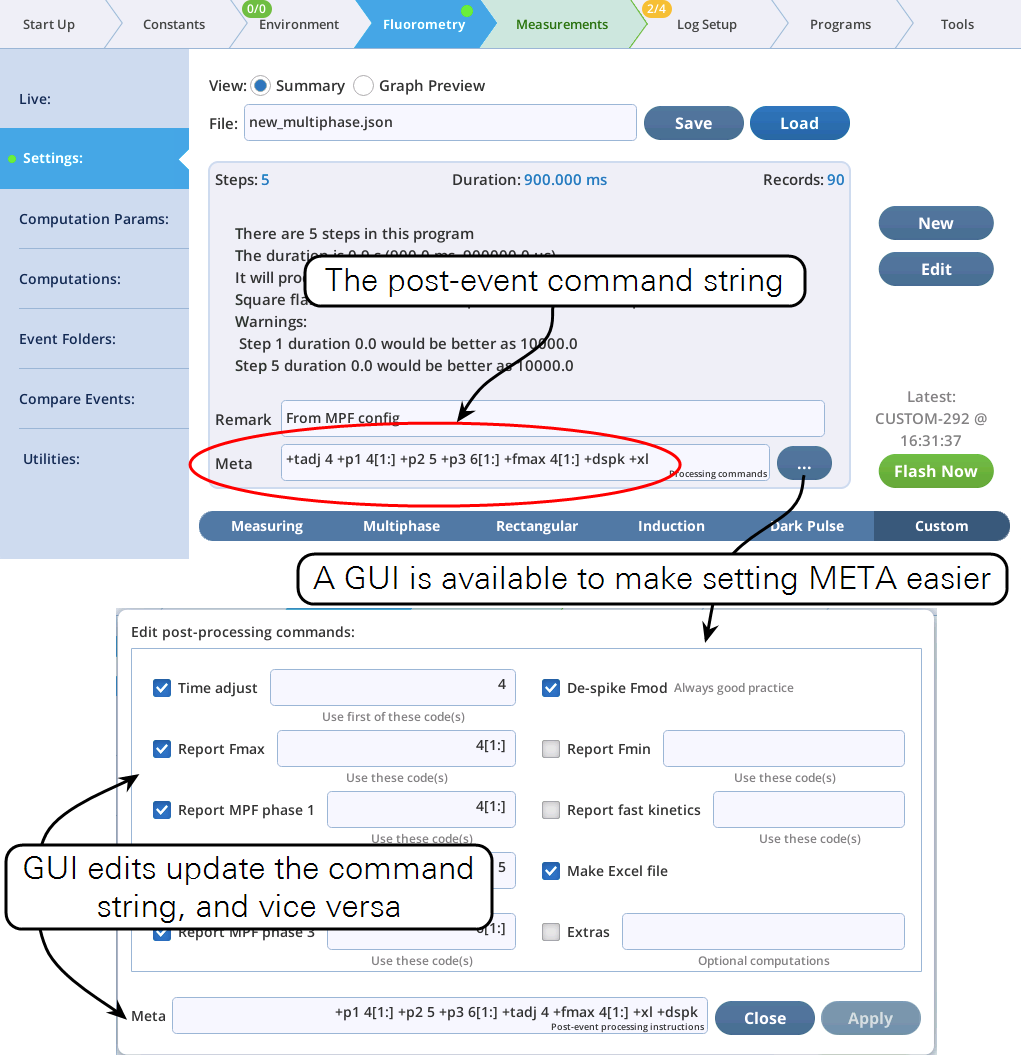
Most Meta commands involve step code numbers, (i.e., the Code column in the Table Editor, is shown to the right). For example, to nd the maximum fluorescence reported from a flash during codes 20 and 21, then either include +fmax 20,21 as part of the Meta string, or use the GUI and do this:

Code specifiers

Code number(s) represent a list of indices. For example, consider a hypothetical flash data set that includes these time series data:

Consider the meta command +fmax 17. The code specifier is 17. This means whatever operation we do will be on data whose 0-based indices (potentially 0 thru 9) are where CODE is 17. The list of indices (starting at 0) where this condition is true is [2, 3, 4, 5, 6] +fmax means we are looking at the FLUOR values, which, for those indices are [93, 94, 95, 96, 97], so, +fmax 17 will return 97, since it is looking at FLUOR values of [93,94,95,96,97].

Similarly, +fmax 16,18 uses indices of [0, 1, 7, 8, 9] an the maximum of those values is 100.

Code specifiers can include slice information (using the Python slicing convention), allowing you to further prune the list of indices. The syntax is (no spaces!)

code[start:stop:step]

where code is the code number (or * for all codes), start is starting index, defaults to 0, stop is stopping index, defaults to None, and step is the step count, defaults to 1. start and stop can be positive (count from the left end) or negative (count from the right end).

Examples using the above hypothetical flash data are shown in Table 8‑16.

Table 8‑16. Code specifier examples and results.

Specifier	Resulting Indicies	Description
16,17,18	[0, 1, 2, 3, 4, 5, 6, 7, 8, 9]	Use just those three codes
*	[0, 1, 2, 3, 4, 5, 6, 7, 8, 9]	Use everything
17	[2, 3, 4, 5, 6]	All code 17s
17[1:]	[3, 4, 5, 6]	Skip the first one
17[:-2]	[2, 3, 4]	Skip the last 2
17[0:4]	[2, 3, 4, 5]	Use only the first 4
17[::2]	[2, 4, 6]	Use every other one
16[-1:],18[:-1]	[0, 9]	Use first of 16, last of 18

Skipping data points is a good way to avoid unwanted biological effects or potential instrument artifacts, such as uncorrected spiking (Despiking modulated fluorescence).

Standard meta commands

Table 8‑17 summarizes the standard meta commands available for use.

Table 8‑17. Meta commands.

Command	Description	Output lines added to file
+tadj codes	Adjusts time (SECS vector) so zero corresponds to the flash (or actinic off).	SECS vector adjusted. The adjustment is recorded by adding an entry like this: "T OFFSET": 1.003675
+dspk	Perform despiking of FLUOR	Any changes to FLUOR are recorded by two lists: the indicies changed, and the old values: "Dspk indices":[35, 70] "Dspk values":[-95727, -95626],
+fk codes	Add fast kinetics for code(s)	"FKdata":"3", "Dur":0.593714, "Fo":748.8, "DCo":7.7288, "InitSlope":49586.0, (If duration greater than 1 ms) "F1":2609.7275, "T@F1":0.00100825, "T@HIR":0.00015225, (If duration greater than 50 ms) "F2":3523.264, "T@F2":0.02411225, "DCmax":39.727, "T@DCmax":0.201712249, "PhiPS2 dc":0.805,
+p1 codes	MPF phase 1 code(s)	"P1 MAXF":1848.65, "T@P1 MAXF":0.09, "Q@P1 MAXF":10348.5, If there is a Phase 2, these are added: "P1 PREDF":1836.69, "P1 DELTAF":-18.77,
+p2 codes	MPF phase 2 code(s)	"P2 SLP":-43.03250083217624, "P2 INT":1878.2743880017254, "P2 R2":0.9280225629842919, "P2 SLP SE":2.2648346023103896, "P2 INT SE":2.5224704199843213, "P2 DQDT":-8515.851835372647,
+p3 codes	MPF phase 3 code(s)	"P3 MAXF":1817.92, "T@P3 MAXF":0.63, "Q@P3 MAXF":10348.3, If there is a Phase 2, these are added: "P3 PREDF":1836.69, "P3 DELTAF":-18.77,
+fmax codes	FMax, QMax for code(s)	"FMAX":1790.33, "T@FMAX":0.00068625, "QMAX":15654.6, "Fs":761.2,
+fmin codes	FMin, Qmin for code(s)	"FMIN":721.27, "T@FMIN":3.59000225, "QMIN":0.00999929, "Fs":761.2,
+xl	Create an Excel file

+tadj (Time adjust)

As reported by the fluorometer (see, for example, Listing 8‑2), the values in the time vector (SECS) start at 0. The +tadj command allows you to shift that time so it corresponds to something else. In the standard flashes, time is adjusted so 0 occurs at the start of the flash, skipping over any margin points. For a dark pulse, time = 0 is when the actinic turns off. In a custom flash you can make time 0 correspond to the first occurrence of a record with the code value of your choice.

See Time adjust to start of flash.

Examples:

+tadj 20	Make time = 0 correspond to the first record of code=20
+tadj 13,14	If multiple codes are given, the one that occurs first is used. If slice specifiers are included (e.g. 4[1:], they are ignored by tadj.

If slice specifiers are included (e.g., 4[1:]), they are ignored by tadj.

If a time shift is implemented, the offset used is recorded (in s) in the file as

+dspk (De-spike)

If the actinic light changes significantly from one step to the next, it usually generates a spurious modulated fluorescence reading (in the FLUOR vector in the file). Despiking replaces those readings with the mean of adjacent readings, to prevent contaminating subsequent computations or interfering with graph scaling.

Examples:

+dspk

Despike FLUOR data

If any values are replaced by despiking, the index of the value replaced, as well as the original replaced value are reported the file in space-delimited strings:

+fmax (Maximum Fluorescence)

To find the maximum modulated fluorescence, use this command.

Examples:

+fmax 4[1:]	Find max FLUOR when code=4 (ignoring  first point)
+fmax 17,20[2:],31	Find max FLUOR in these codes

The following entries are added to the file that contain the results: the maximum (FMAX), and also the corresponding time and quantum values.

The reported value FMAX is actually the average of three data points: the actual max, and the neighbor to each side (or the two neighbors on one side, if the maximum occurs at the end of a code segment).

If the processing codes include the +p2 command (MPF Phases 2), then only FMAX is reported, with the value coming from the P2 INT value (or, if there is also a +p1 command, the maximum of P2 INT and P1 MAXF.

+fmin (Minimum Fluorescence)

To find the minimum modulated fluorescence, use this command.

Examples:

+fmin 21	Find min FLUOR when code=3
+fmin 20,21	Find min FLUOR when code is 20 or 21

The following entries are added to the file that contain the results: the maximum (FMIN), and also the corresponding time and quantum values.

The reported value FMIN is actually the average of three data points: the actual min, and the neighbor to each side (or the two neighbors on one side, if the minimum occurs at the end of a code segment).

+p1 (MPF Phase 1)

To analyze part of a flash event as an MPF phase 1, use this command, specifying which code(s) are to be included.

Examples:

+p1 4	Consider code 4 to be Phase 1
+p1 20,21,22	Consider codes 20, 21, and 22 to all be part of Phase 1

The following is added to the file:

If there is also a Phase 2 associated with the flash, the following will also be added, based on the t of F vs 1E4/PFD done in Phase 2:

+p2 (MPF Phase 2)

To analyze part of a flash event as an MPF phase 2, use this command, specifying which code(s) are to be included.

Examples:

+p2 5	Consider code 5 to be Phase 2
+p2 24,25,26	Consider codes 24, 25, and 26 to all be part of Phase 2

The following is added to the file:

+p3 (MPF Phase 3)

To analyze part of a flash event as an MPF phase 3, use this command, specifying which code(s) are to be included.

Examples:

+p3 6	Consider code 6 to be Phase 3
+p2 27,28	Consider codes 27 and 28 to all be part of Phase 3

The following is added to the le:

If there is also a Phase 2 associated with the flash, the following will also be added, based on the fit of F vs 1E4/PFD done in phase 2:

+fk (Fask Kinetics)

Fast Kinetics refers to the computations associated with the initial rise of an induction curve.

To do the complete analysis, durations of at least 0.01s are required.

Examples:

+fk 3	Use code 3 for computing fask kinetics
+fk 31,32,33	Use code 31, 32, and 33 for computing fask kinetics

+xl Make Excel File

Creates an Excel file, in addition to the .json file.

Meta extras

When the meta parser encounters a "non-standard" meta specifier (i.e., anything that is not in Table 8‑17), it is considered an "extra" meta command. On the user interface, extras show up as shown in Figure 8‑68.

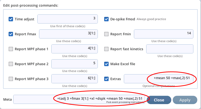
There are several such commands that the basic system supports (Table 8‑18), and it is possible to add user defined extras as well (see User-defined meta extras). But first, let's consider the two in Figure 8‑68:

+mean 50 +max(,2) 51.

The first looks like other meta commands, but the second (+max(,2) 51) is an example of the optional parameters available to meta extras. These are described next.

Optional parameters

As you might guess, +mean 16 computes the mean value of FLUOR for code 16 data. But what if you want the mean of light (PFD), or non-modulated fluorescence (DC) instead? Meta extras can pass parameters by appending them in a comma separated list (no spaces!) after the name, surrounded with ( ). In the case of +mean, it supports one optional parameter, an alternative target (any of the time series variables in a flash file).

+mean(dc) 17 - compute the mean of DC values for code 17.

As a convenience, you don't need to specify a target in upper case (DC), although you can; the code supporting

+mean will turn dc into DC for you.

In the case of max(,2) 51, there are two parameters supported: target, and count. +max finds the maximum value of target, then averages some neighboring values (count values on either side) and returns that value.

Thus +max with no code will find the maximum FLUOR value for an entire flash, and no averaging. +max(,2) 51 will find the maximum value of FLUOR for code 51, averaged with the two values before and after. And +max(dc/q,1) 51 will find the maximum value of DC/Q for code 51, averaged with one value before and after.

Standard extras

The following illustrates the syntax we'll use for describing extra commands, where square brackets [ ] mean "optional".

+name codes - name requires codes

+name[(arg1,arg2)] [codes] - name has 2 optional parameters, arg1 and arg2. codes is optional.

Table 8‑18 summarizes the meta extras the system provides, with details in the sections following. If you don't find what you need here, then User-defined meta extras shows how to add your own.

Table 8‑18. Meta extra commands

Command	Description	Defaults	Output Examples
+fit[(y tar, x tar, pow)] [codes]	Polynomial fit	y tar = fluor x tar = secs, pow = 1 codes = *	"fit 16":[-32.88, 980] "fit(dc,pfd,2) 5": [2.504e-05, 7.212, 191.5]
+iv[(target, power)] [codes]	Initial value	target = fluor power = 1 codes = *	"iv 16":21.43 " iv(dc/q) 16[2:]":29.51
+max[(target, intrvl)] [codes]	Maximum	target = fluor intrvl=0 codes = *	"max 16":123.45 "max(,2) 16":130.33 "max(dc/q) 16[2:]":21.34
+mean[(target)] [codes]	Mean	target = fluor codes = *	"mean 16":1234.56 "mean(dc/q) 16[2:]":18.46
+min[(target, intrvl)] [codes]	Minimum	target = fluor intrvl=0 codes = *	"min 16":123.45 "min(,2) 16":130.33 "min(dc/q) 16[2:]":21.34
+smean[(target, slice1, slice2)] [codes]	Mean of sorted (low to high) data. Slicing option provided.	target = fluor slice1 = 0 slice2 = None codes = *	"smean(dc/q,1:-1) 16":10.154, "smean(,-10) 16":644.132
+stats[(target)] [codes]	Combines five basic stats into one command	target = fluor codes = *	"count(dc) 16":10, "min(dc) 16":10567.6, "max(dc) 16":10600.5, "mean(dc) 16":10584.50, "std(dc) 16":9.19
+std[(target)] [codes]	Std dev	target = fluor codes = *	"std 16":12.34 "std(dc/q) 16[2:]":8.23

+fit

Compute the coefficients of a polynomial fit.

+fit[(y target, x target, power)] [codes]

target - can be any time series ID in the file (SECS, FLUOR, DC, PFD, RED, REDMODAVG, FARRED, CODE or one of the computed light values BLUE or DC/Q). (target can be entered as lowercase.) If not specified, target defaults to FLUOR.

x target - can be any time series ID. If not specified, target defaults to SECS.

codes - see Code specifiers. If not specified, defaults to * (all data)

Examples:

+fit 22[2:]	Generate a linear fit of FLUOR vs SECS for the code 22 data, neglecting first two points in the fit. Report the slope of the fit.
+fit(dc) 22[2:]	Same as first, except fit DC instead of FLUOR

The list of fit parameters added to the file uses the extras specifier as the label: For example, fit(dc,pfd,2) 5 will yield a list of coefficients, highest order first.

+iv

Initial Value: Fit a polynomial as a function of time, nd the value at the start of a step.

+iv[(target,power)] [codes]

The polynomial is evaluated at the start of the rst step specified in codes.

target - can be any time series ID in the file (SECS, FLUOR, DC, PFD, RED, REDMODAVG, FARRED, CODE or one of the computed light values BLUE or DC/Q). (target can be entered as lowercase.) If not specified, target defaults to FLUOR.

power - the power of the fit. Default is 1.

codes - see Code specifiers. If not specified, defaults to * (all data)

Examples:

+iv 22[2:]	Generate a linear fit of FLUOR vs SECS for the code 22 data, neglecting first two points in the fit.
Evaluate at time of the start of first code 22 step.
+iv 22[2:],23	Same as above, but include code 23 data as well.
+iv 23,22[2:]	Same as above, except now the  t is evaluated at the  first code 23 step.
+iv(,2) 22[2:]	Same as  rst example, but use a 2nd order polynomial.
+iv(dc) 22[2:]	Same as  rst, except  t DC instead of FLUOR

The initial time t0 of a step is computed from the SECS value for that step, adjusted for the modulation and output rates. See Fluorometry timing details.

The entry added to the file uses the extras specifier as the label: For example, iv 3[2:] will yield

+max

Find the maximum, with option to average adjacent points.

target - can be any time series ID in the file (SECS, FLUOR, DC, PFD, RED, REDMODAVG, FARRED, CODE or one of the computed light values BLUE or DC/Q). (Target can be entered as lowercase.) If not specified, target defaults to FLUOR.

interval - default is 0. Number of data values on each side of the maximum value to average together for the result.

codes - see Code specifiers. If not specified, defaults to * (all data)

Examples:

+max 20,22[2:]	find the maximum of FLUOR for the specified codes.
+max(,2) 16	find the average of 5 data points centered on the maximum value of FLUOR in code 16 data.
+max(dc) 16	find the highest value of DC in code 16 data

The entry added to the file uses the extras specifier as the label: For example, max(,2) 3[1:] will yield

+mean

Compute the mean value.

target - can be any time series ID in the file (SECS, FLUOR, DC, PFD, RED, REDMODAVG, FARRED, CODE or one of the computed light values BLUE or DC/Q). (Target can be entered as lowercase.) If not specified, target defaults to FLUOR.

codes - see Code specifiers. If not specified, defaults to * (all data)

Examples:

+mean 20,22[2:]	compute mean of FLUOR for the specified codes.
+mean(dc) 16	compute the mean of DC all code 16 data.

The entry added to the file uses the extras specifier as the label: For example, mean 3[2:] will yield

+min

Find the minimum, with option to average adjacent points.

target - can be any time series ID in the file (SECS, FLUOR, DC, PFD, RED, REDMODAVG, FARRED, CODE or one of the computed light values BLUE or DC/Q). (target can be entered as lowercase.) If not specified, target defaults to FLUOR.

interval - default is 0. Number of data values on each side of the minimum value to average together for the result.

codes - see Code specifiers. If not specified, defaults to * (all data)

Examples:

+min 20,22[2:]	find the minimum of FLUOR for the specified codes.
+min(,2) 16	find the average of 5 data points centered on the minimum value of FLUOR in code 16 data.
+min(dc) 16	find the lowest value of DC in code 16 data

The entry added to the file uses the extras specifier as the label: For example, min(,2) 3[1:] will yield

+smean

Sorts the data (low to high) then does the mean value of the selected slice (uses Python list slicing) of that data.

target - can be any time series ID in the file (SECS, FLUOR, DC, PFD, RED, REDMODAVG, FARRED, CODE or one of the computed light values BLUE or DC/Q). (target can be entered as lowercase.) If not specified, target defaults to FLUOR.

slice1 - post-sort slice parameter #1. Defaults to 0

slice2 - post-sort slice parameter #2. Defaults to None

codes - see Code specifiers. If not specified, defaults to * (all data)

Examples:

+smean(,2,-1) 44	Get mean of FLUOR for code 44 data, neglecting the lowest 2 and highest 1 values.
+smean(dc,-10) 3	Get mean of the highest 10 values of DC for code 3 data.
+smean(dc,0,10) 3	Get mean of the lowest 10 values of DC for code 3 data.
+smean(,0,10) 3[2:-1]	Using all of the code 3 FLUOR data except the  rst 2 and  nal points, sort it, then get the mean of the lowest 10 points.

Note: there is potentially slicing done before the sorting, and that is specified in the code specifier. The slicing specified in the optional parameters is done after the sorting. The last example above illustrates this point.

The entry added to the file uses the extras specifier as the label: For example, smean(,0,10) 3 will yield

+stats

Find count, min, max, mean, and standard deviation for a code. +stats can be a convenient shortcut instead of specifying +min +max +mean +std.

target - can be any time series ID in the file (SECS, FLUOR, DC, PFD, RED, REDMODAVG, FARRED, CODE or one of the computed light values BLUE or DC/Q). (target can be entered as lowercase.) If not specified, target defaults to FLUOR.

codes - see Code specifiers. If not specified, defaults to * (all data)

Examples:

+stats 51	Get stats on FLUOR for all points with code 51. +stats(dc) 16 - Get stats on DC for all points with code 16.
+stats	adds 5 lines to the  le, none of which are labelled stats:

+std

Compute the standard deviation.

target - can be any time series ID in the file (SECS, FLUOR, DC, PFD, RED, REDMODAVG, FARRED, CODE or one of the computed light values BLUE or DC/Q). (target can be entered as lowercase.) If not specified, target defaults to FLUOR.

codes - see Code specifiers. If not specified, defaults to * (all data)

Examples:

+std 20,22[2:]	find the standard deviation of FLUOR for the specified codes.
+std(pfd) 16	find the highest value of PFD in code 16 data

The entry added to the file uses the extras specifier as the label: For example, std 3[2:] will yield