This section introduces some basics related to the fluorometer and fluorescence measurements. Here we offer some protocols for determining the best settings when using the fluorometer, followed by Fluorescence measurement examples.
When you are operating your 6800-01/A for the first time or working with a new species it is important that you configure your fluorometer settings properly. Starting with the default settings is a good idea, but you should optimize them for your specific leaves for best results.
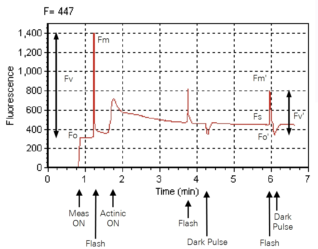
Figure 8‑27. Example measurements of chlorophyll a fluorescence parameters of a dark-adapted leaf following a few minutes of exposure to actinic light.
Once you determine which fluorescence parameters are of interest to you (e.g., Fv/Fm,ΦPSII), evaluate which fluorescence settings are important to optimize. For instance, if you are only interested in light-adapted ΦPSII, then you do not need to optimize the dark-adapted settings (Dark mod rate) or the Dark Pulse settings.
The measuring beam
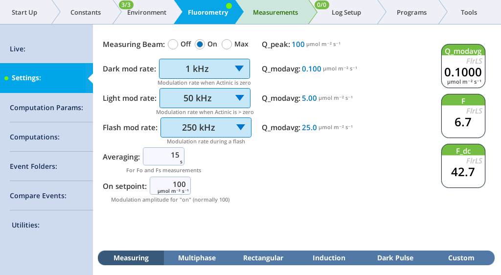
The measuring beam is used to probe fluorescence. It is weak, modulated (turned on and off) light with a peak intensity (Q_peak) of 100 μmol m-2 s-1, but an average intensity (Q_modavg) that varies depending on the modulation rate (mod rate) (see Table 8‑8).
Table 8‑8. Examples of measuring beam modulation rates and their resulting Q_modavg (in μmol m-2 s-1).
Mod rate
Q_modavg
10 Hz
0.001
1 kHz
0.1
10 kHz
1
50 kHz
5
250 Hz
25
The measuring beam should be optimized for which conditions you are measuring, dark- or light-adapted (Figure 8‑27). If measuring under both dark and light-adapted conditions, optimize for both since the fluorometer will switch modulation rate based on whether actinic light is turned on or off.
Dark mod rate
The Dark mod rate will be used when the fluorometer actinic light setpoint is off or close to 0 μmol m-2 s-1. At higher modulation frequencies, the fluorescence signal-to-noise ratio will be better. However, high frequencies also increase the average irradiance (Q_modavg; see Table 8‑8). If Q_modavg is too high, the modulated light can become actinic (drive photochemistry), so the best Dark mod rate is the highest rate without this affect.
An experiment with example results to find the optimal Dark mod rate is described here:
Dark-adapt your leaf.
Dark-adapt the leaf overnight (alternatively, for a few hours in a dark room).
Environmental controls.
Set up Environmental controls (if a control is not mentioned below you can leave it turned off):
Flow: 600 μmol s-1
Light: Off
Fluor: Set Measuring Beam to Off
Clamp on to the dark-adapted leaf.
Go to the Fluorometry tab > Utilities/Test. In the drop down menu, select Test Dark Mod Rates and tap Start.
The program will sequentially increase the measuring beam modulation rate while turning the modulation beam off between setpoints to allow any induced photochemistry to relax.
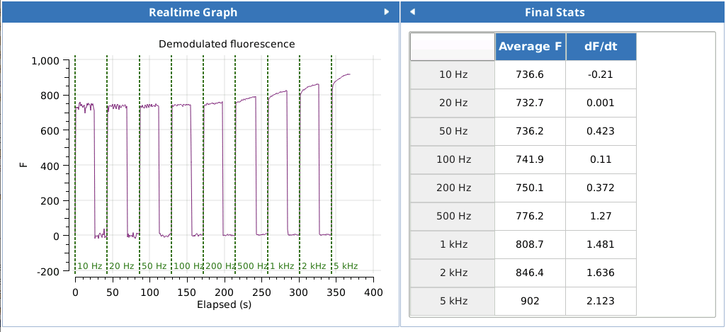
The graph will display real-time demodulated fluorescence where green markers will indicate what modulation rate is being applied. As the program progresses, the table will populate with values. See our example results from clamping onto a dark adapted house plant below.
Figure 8‑28. Fluorescence from leaf with increasing Dark mod rate. At 200 Hz we start to see an increase in F, indicating photochemistry. A good Dark mod rate for this plant would therefor be 100 Hz.
Light mod rate
The Light mod rate is the modulated rate when actinic light is turned on. If you are working at light intensities greater than 50 μmol m-2 s-1, we recommend setting the Light mod rate to 50 kHz for the best signal-to-noise ratio. At low actinic light, use ≤10 kHz Light mod rate (see Table 8‑8).
Flash mod rate
The default Flash mod rate is 250 kHz. Use this rate for best signal-to-noise ratio.
Averaging
Fo and Fs parameters are determined from the de-modulated fluorescence signal (F) averaged over the Averaging duration, as set on the Measuring tab. After clamping onto your leaf during dark-adapted and survey measurements, you need to wait the additional Averaging time before logging Fo and Fs. If you do not wait long enough after clamping on a leaf, your average fluorescence readings will include data prior to chamber closure, resulting in artificially high Fv/Fm or ΦPSII values.
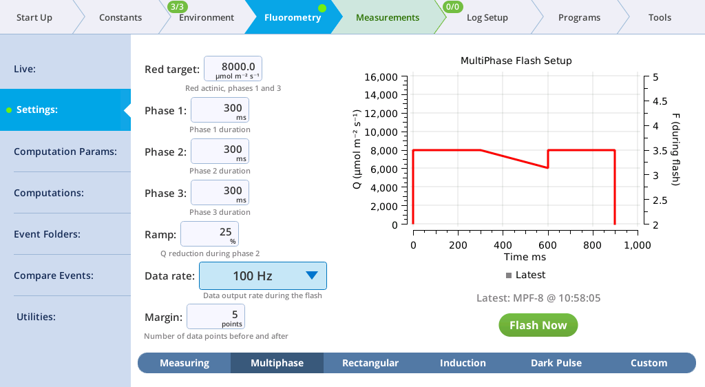
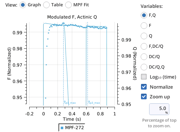
The defaults for phase 1, phase 2, and phase 3 are 300 ms. This is usually a good default. You want to make sure phase 1 is long enough to capture Fmax. Time when Fmax occurred in phase 1 (T@P1_FMAX) can be found in the individual flash files recorded when doing the experiment under Rectangular flash optimization experiment for the Rectangular flash. Adjust phase 2 and 3 durations so that the plateaus of phase 1 and phase 3 fluorescence are the same (P3_deltaF = 0). See examples of good and bad flash data in Figure 8‑29.
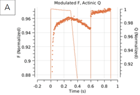
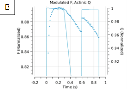
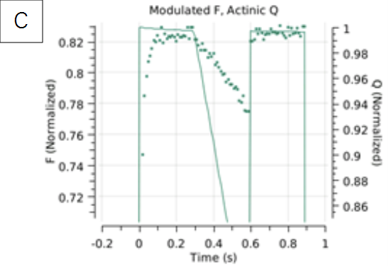
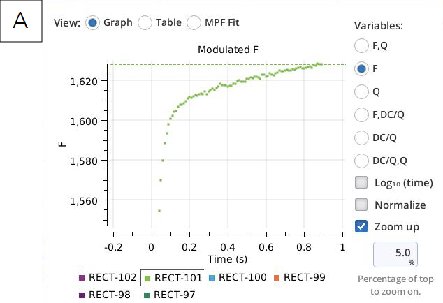
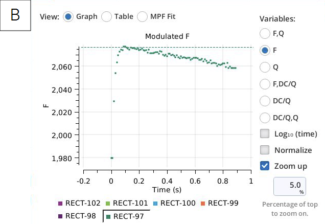
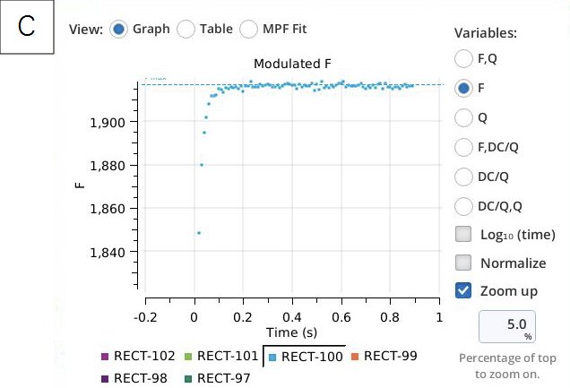
Figure 8‑29. (A) Red target too low. P3_deltaF = 34.12. (B) P3_deltaF = -20.86. Shorten phase 1, 2, and 3, alternatively play around with lowering the flash intensity. (C) Good looking MPF. P3_deltaF = 1.67.
Ramp
The Ramp determines the % decrease in light during phase 2. A good starting ramp value is typically between 15 and 40%. See Loriaux et al. 2013 (3) for more details on the impact of ramp rate.
Data rate and margin
You do not need to change these. Higher data rates will produce noisier data and the purpose of the margin is to help visualize the flash when looking at the data in the Results or Files tabs.
Multiphase flash optimization experiment
Here is an experiment with sample data to show an MPF optimization procedure:
Pick a red target.
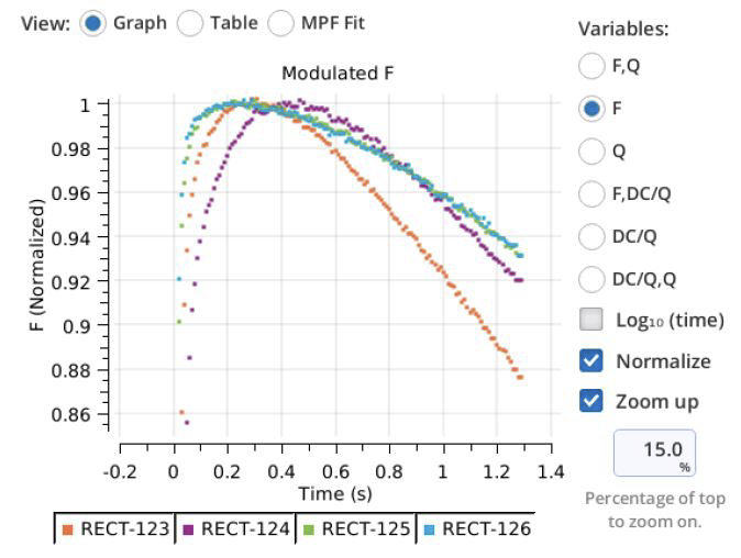
Follow the steps under the Rectangular flash optimization experiment. Measuring a greenhouse-grown sunflower with the following settings: max = 10,000 μmol m-2 s-1, min = 6,000 μmol m-2 s-1, duration = 1300 ms and four flashes provided the following results:
In this example, RECT-125 (10,000 μmol m-2 s-1) and RECT-126 (8,000 μmol m-2 s-1) were the best red targets. Why? They both had rapid initial rise and the least amount of flash-induced quenching. Maximal fluorescence (T@FMAX) occurred at about 250 ms.
Pick durations.
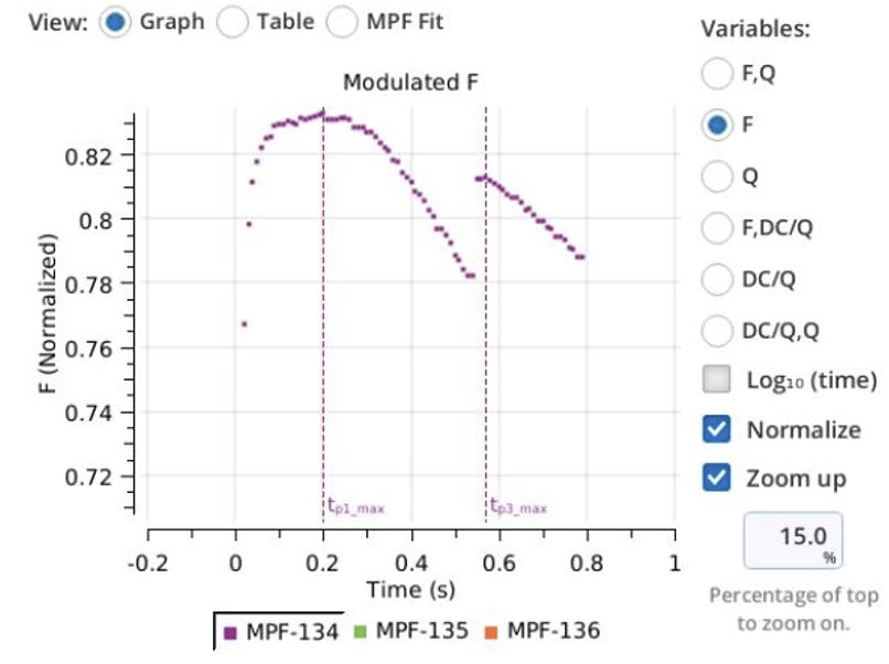
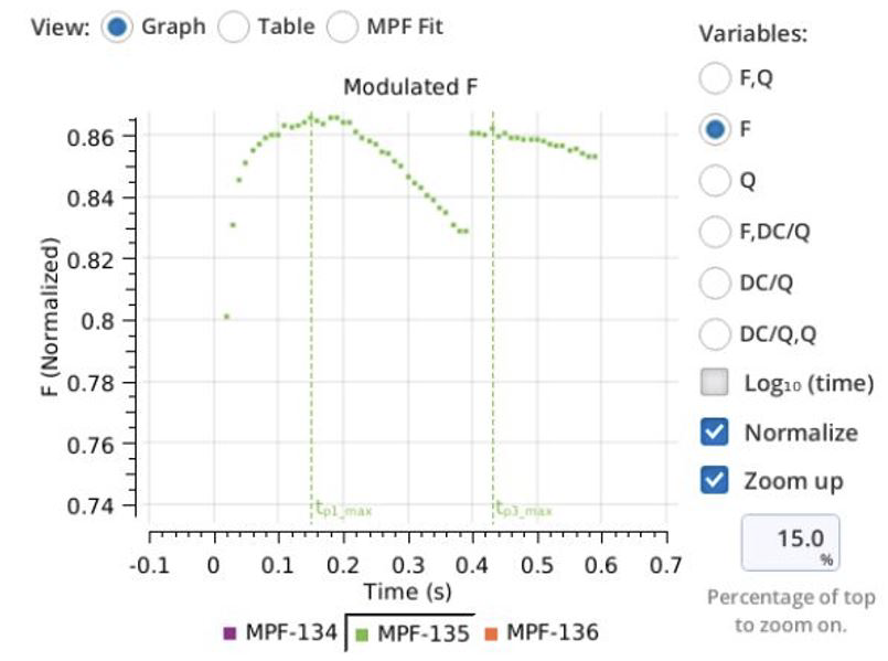
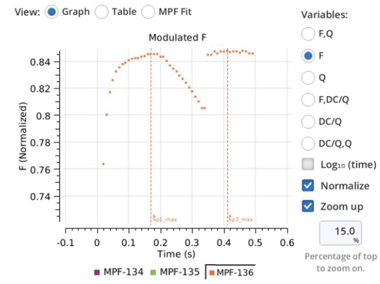
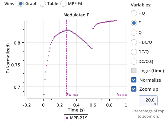
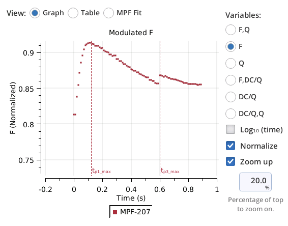
Based on the results from step 1 we picked a red target of 8,000 μmol m-2 s-1, a ramp rate of 25% (good default), and phase 1 = 300 ms, phase 2 = 250 ms, and phase 3 = 250 ms:Figure 8‑30. P3_deltaF = -27.93.
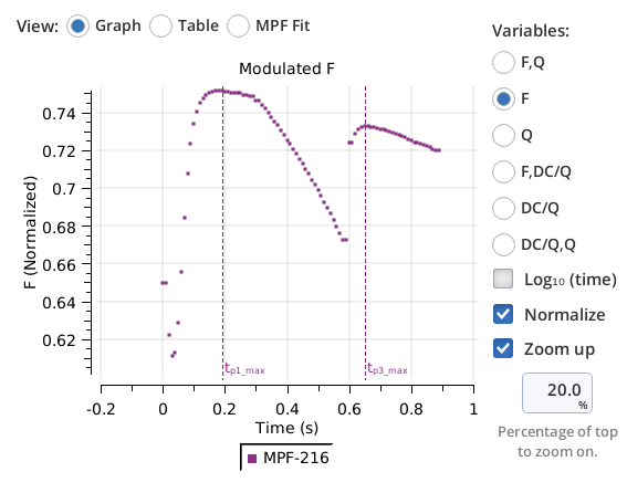
Since P3_deltaF in Figure 8‑30 was large and T@P1_MAXF occurred at 200 ms we reduced each of the phase durations to 200 ms:Figure 8‑31. P3_deltaF = -8.72.MPF-135 (Figure 8‑31) still shows an offset in P3_deltaF (8.72) so we reduce the phase 2 and 3 durations to 150 ms each:Figure 8‑32. P3_deltaF = 1.67.
We have found a good set of MPF settings for this particular plant.
Examples of bad multiphase flash data
The following examples of bad data may be solved by the accompanying advice.
Small phase 2 slope (P2_SLP) and low P2_R2?
Figure 8‑33. P2_SLP = -12.4 and P2_R2 = 0.722.
Issue: Red target is too high so light is saturating even when Q is ramping down. Common for plants grown in low light conditions.
Solution: Lower the red target or do a rectangular flash.
Continuous increase in fluorescence and large positive P3_deltaF?
Figure 8‑34. P3_deltaF = 31.6.
Issue: Red target is too low.
Solution: Increase red target.
Continuous decrease in fluorescence and T@P1_MAXF much shorter than phase 1 duration?
Issue: Phase 1 and/or phase 2 are too long or red target is too high.
Solution: Shorten the phase durations and/or lower red target.
The rectangular flash
Red target
The default in the 6800-01/A is 10,000 μmol m-2 s-1. This setting should be verified on your leaves before you begin. Test higher and lower targets and check your data. Rectangular flash optimization experiment shows how to use the Test Flash Intensities program to find your optimal red target. Pick the lowest red target above which Fmax does not significantly increase. See examples of good and bad flash data in Figure 8‑37.
Figure 8‑37. (A) 3,000 μmol m-2 s-1. The red target is too low, indicated by the slow rise and fluorescence never saturates. (B) 12,500 μmol m-2 s-1. The red target is too high (or the duration is too long, see Duration) which causes flash-induced quenching. This can sometimes happen at lower red targets if the leaf recently experienced a flash. Be sure to leave enough time for flash-induced quenching to relax before giving another flash. (C) 8,700 μmol m-2 s-1. The red target is good, indicated by the rapid rise to steady fluorescence.
Note: Evaluate Q before you look at fluorescence data. If Q is not rectangular, fluorescence won't be either. In it is not rectangular when zoomed in to 5% , then perform the square flash correction, described on The square flash correction.
Duration
Durations between 700-1200 ms are typically recommended. After you have set the proper red target, look at the Results table (or flash files: directory licor/logs/flrevents) for the parameter T@FMAX (time at maximal fluorescence). If this is always equal to the duration of the flash, your duration may be too short (or your red target too low, see A in Figure 8‑37). If you however start to see a decline in fluorescence after it has plateaued, your duration may be too long (or your red target too high, see B in Figure 8‑37).
Note: Some species will have more flash-induced quenching than others. To optimize a flash you have to find a good balance between the red target and duration settings where flash-induced quenching is minimized.
Data rate and margin
You do not need to change these. Higher data rates will produce noisier data and the purpose of the margin is to help visualize the flash when looking at the data in the Results or Files tabs.
Rectangular flash optimization experiment
The following shows an experiment to find your plant’s optimal red target. We will use rectangular flashes to find the red target for which Fm’ (Fmax) no longer increases with increased intensity.
Environmental controls.
Acclimate the plant at the light intensity and environmental control settings you will be making your measurements at, and Light and Flash mod rates configured as described above.
Clamp on to the light-adapted leaf.
Go to Fluorometry > Utilities/Test. In the menu, select Test Flash Intensities and tap Start.
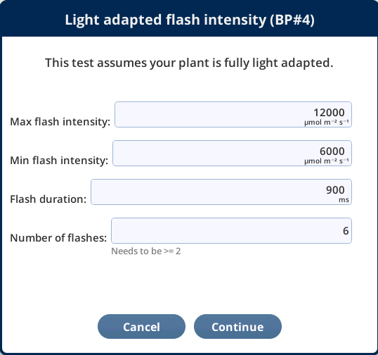
Edit the following dialog.
We suggest keeping a wide range of intensities and about five to eight flashes. Set the duration to around 1000 ms. Here we chose max 12,000 μmol m-2 s-1, min 6,000 μmol m-2 s-1, a duration of 900 ms, and six flashes.
When you are ready to start the program tap Continue. The program will wait for fluorescence to stabilize and then cycle through randomized flash intensities.
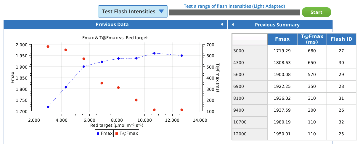
As the program progresses, the graph and table will populate with values. See our example flashes from running the program clamped to a greenhouse grown soybean in Figure 8‑38:
Figure 8‑38. Fmax and T@Fmax from a leaf exposed to flashes with randomized red target setpoints. Based on the graph we would pick a light intensity of about 8,000 μmol m-2 s-1 since increasing the red target past 8,000 did not significantly increase Fmax.
Note: If the highest Fmax occurred at the highest light intensity, or above 10,000 μmol m-2 s-1, we recommend using the multiphase flash.
The square flash correction
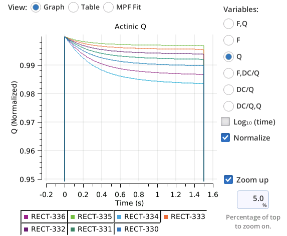
When the LI-6800 fluorometer is performing a flash, the actinic intensity falls off slightly with time. Figure 8‑39 shows a normalized plot of Q for 7 flashes ranging in intensity from 7,000 to 16,000 µmol/m2/s. The decay for a 16,000 flash is typically less than 2% after a second, and about 0.3% for the 7,000 flash. This also depends on the fluorometer's LED tile temperature; the higher the temperature, the more the falloff.
Figure 8‑39. Flash intensity falloff with time depends on the intensity.
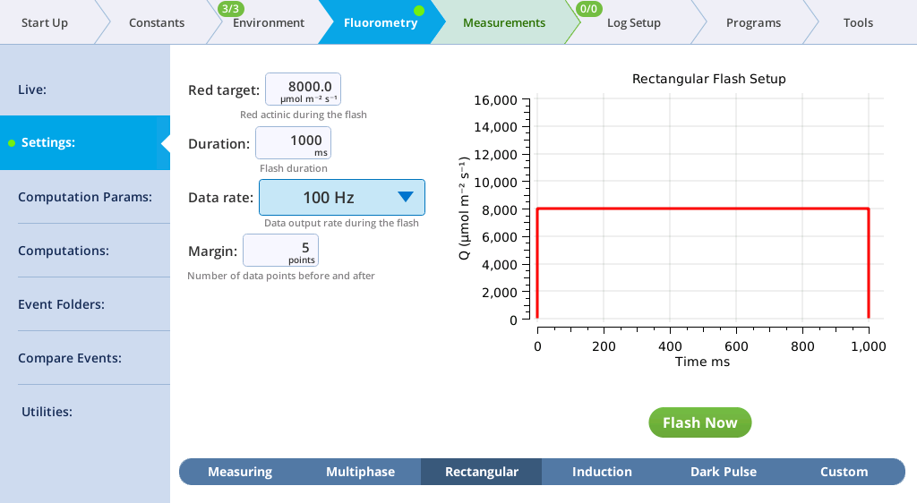
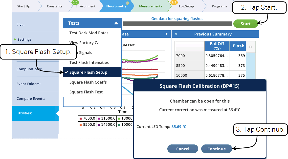
Square Flash Setup
A square flash correction can be implemented by running the Square Flash Setup routine.
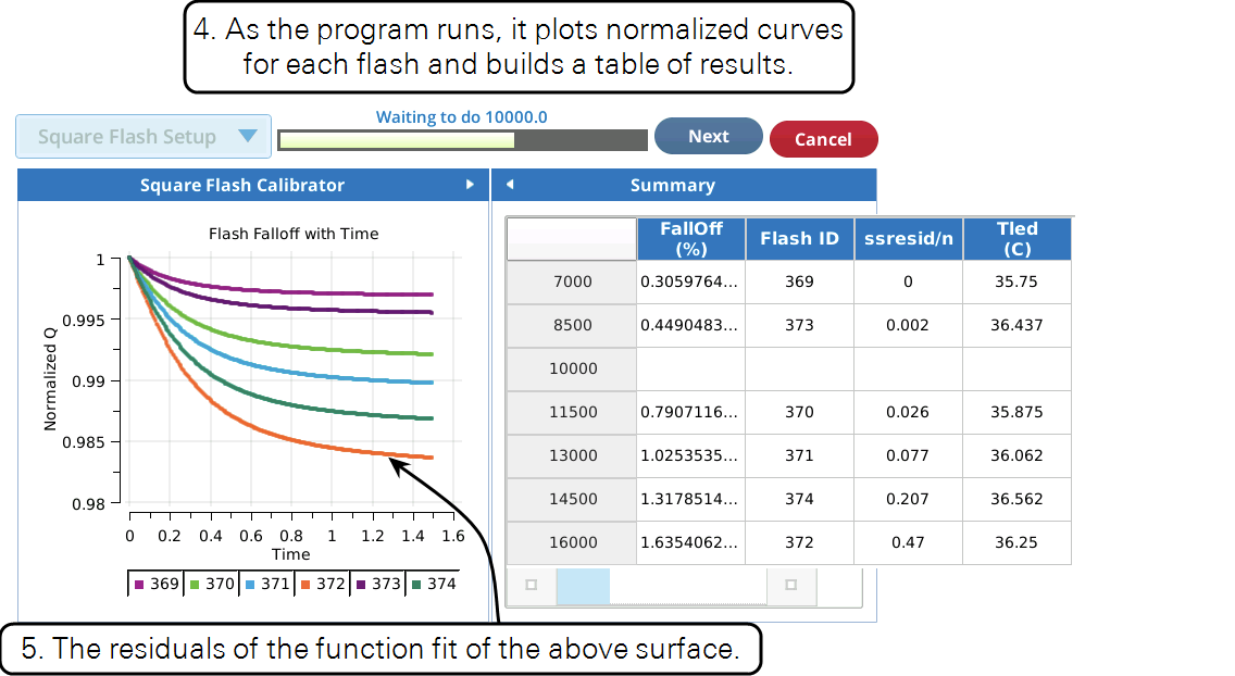
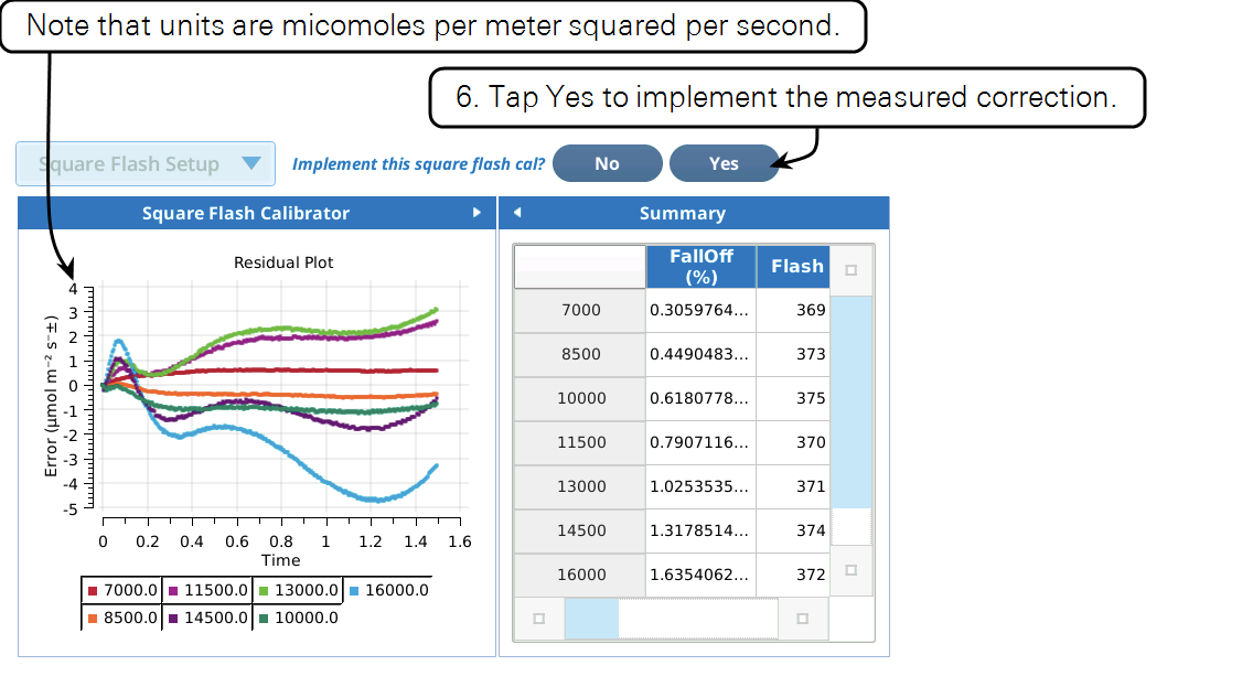
Figure 8‑40. Launching the program that collects data for doing square flash corrections.Figure 8‑41. After collecting the required data, the program present a plot of the residuals, and you can implement the correction function.
Suggested square flash calibration strategy:
Do the calibration with the fluorometer well warmed up, perhaps after leaving the actinic on at 500 or 1000 μmol m-2 s-1 for 30 minutes. Although the calibration does depend on LED tile temperature (FlrLS:Tled), there is a built-in temperature correction that compensates at other temperatures. Use the Square Flash Test (below) to determine how well the calibration is doing at other temperatures, and you can redo the calibration when and if it becomes necessary.
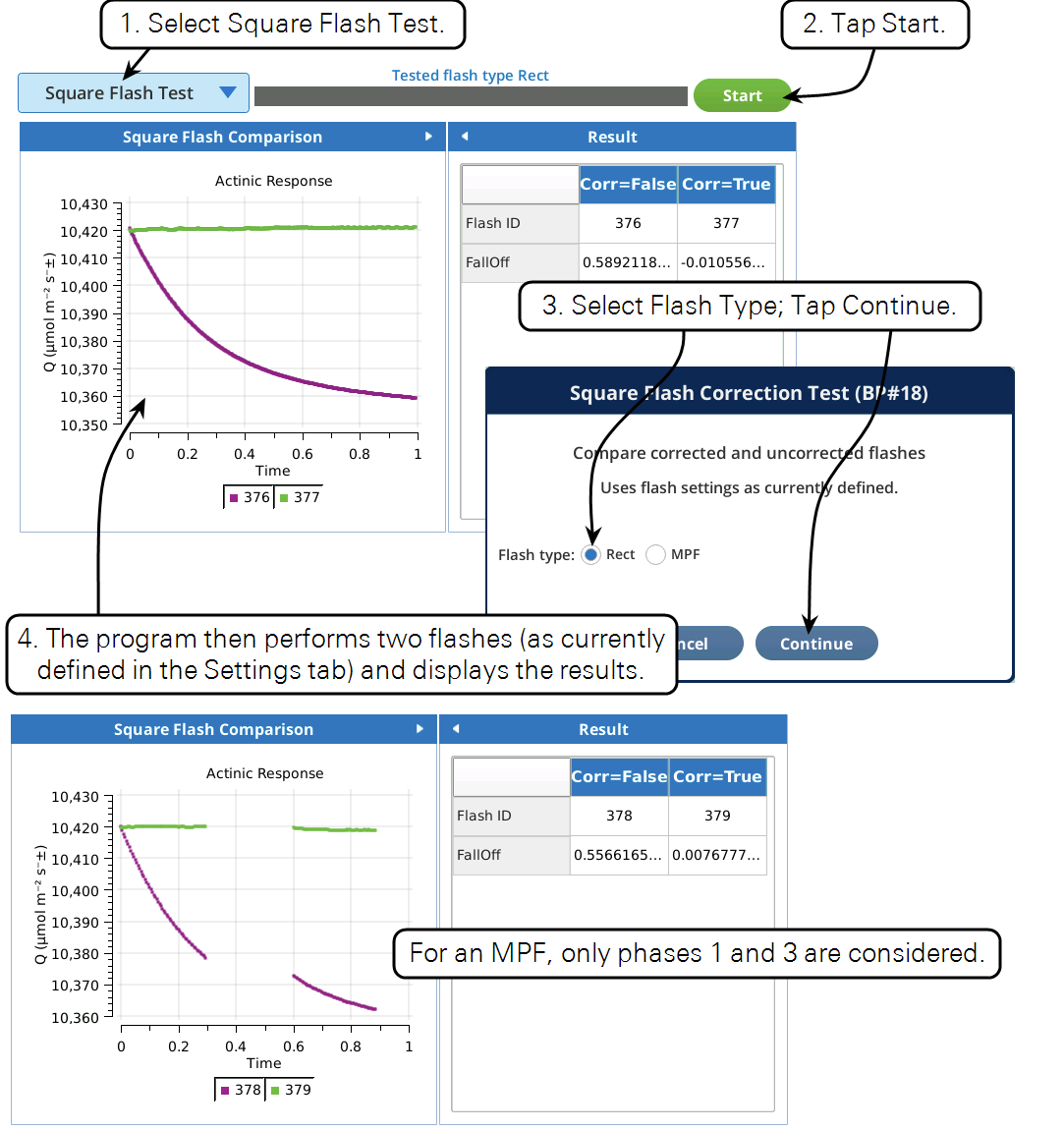
Square Flash Test
A simple way to test how well the square flash correction works is to run the Square Flash Test.
Figure 8‑42. Rectangular and MultiPhase flashes can be tested. The tests simply compares two flashes — with and without correction.
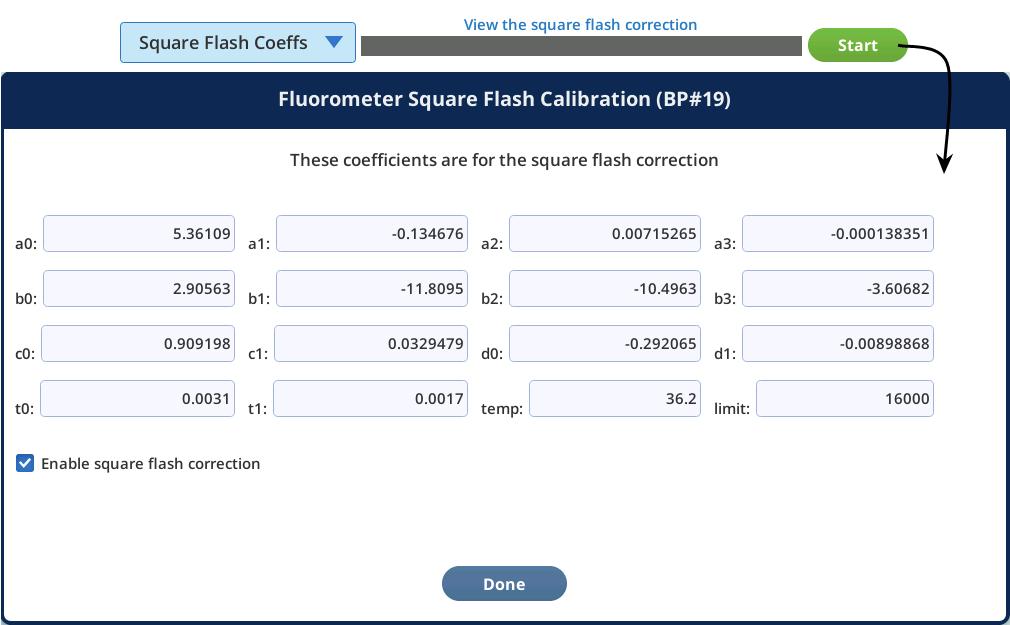
Square Flash Coefficients
You can view the square flash correction coefficients. Note the checkbox that let's you turn them on and off, if you so choose.
Figure 8‑43. Viewing the square flash correction coefficients. They are stored on-board the fluorometer itself.
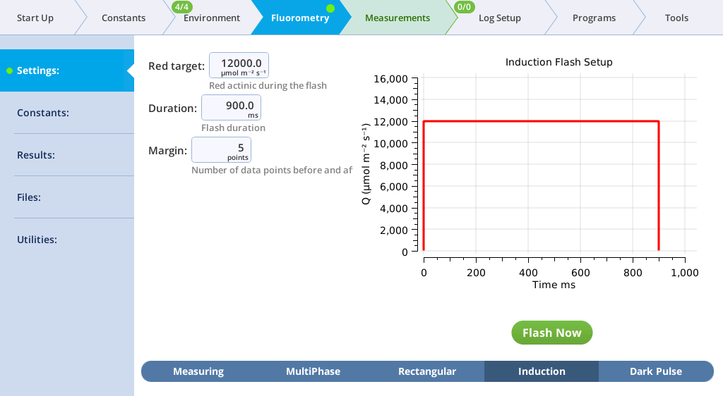
The induction flash
The induction flash is like the rectangular flash in that it gives you a square shaped flash. The difference is that the fluorescence is sampled at a much higher frequency in order to estimate certain kinetics of the fluorescence response (OJIP; origin, inflection, intermediary peak, and peak). The fluorescence response from the flash is plotted vs. time on a log scale where the rise and plateaus of the fluorescence gives information about specific chlorophyll kinetics. The red target and duration considerations are the same as the rectangular flash.
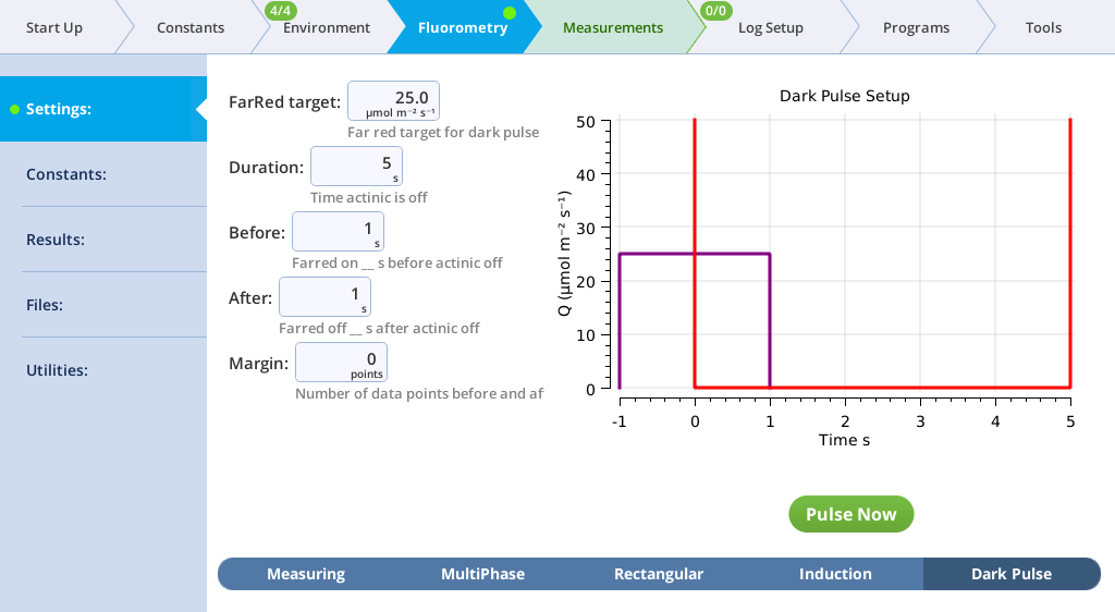
The dark pulse
The dark pulse consists of a brief period of far-red light followed by a few seconds of darkness applied to light adapted leaves to estimate the parameter Fo’. The difference between Fo and Fo’ is that for Fo’, NPQ is still engaged (KNPQ > 0).
8‑22
8‑23
Photochemistry relaxes quickly in the dark, while NPQ is still engaged. Far-red light is used to drive electrons forward to PSI, resulting in fully oxidized QA (QA = 1). The dark pulse is used in flash event 2: FoFm (dark) or FsFm’Fo’ (light) and is applied right after the flash. The resulting Fo’ is used to calculate several parameters related to quenching mechanisms.
There are some assumptions with this method:
When a flash occurs prior to the dark pulse, we do not excessively alter NPQ (purpose of having a short flash and shows the importance of picking an appropriate flash duration), nor does the brief period of darkness during the pulse alter NPQ (2).
The short dark pulse, along with far-red light, is sufficient to completely oxidize QA.
The far-red light, preferentially used by PSI, results in a fully oxidized QA; i.e. the far-red light does not excite any electrons in PSII, which would result in QA < 1. This may or may not be true since far-red light up to 800 nm has been shown to drive PSII electron transfer (3).
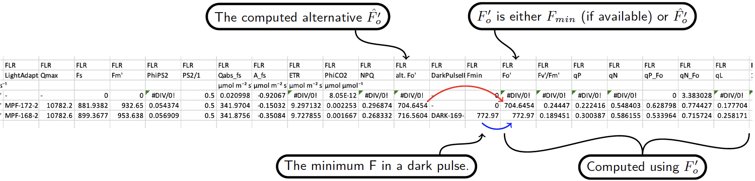
Version 1.5 implements the alternative computation of Fʹo (2) which we will call :
8‑24
Figure 8‑44 illustrates how this handled in practice in the LI-6800. Anytime a light adapted flash is done when dark adapted values (Fo and Fm) are available, is computed, and used for the working value of Fʹo in computing quenching coefficients. If a dark pulse has been performed, its minimum value Fmin is recorded, and that is used for the working value of .
Figure 8‑44. How the alternative Fʹo is used. Note (2nd obs) the quenching computations without doing a dark pulse.
Far red target
The default target value of 25 μmol m-2 s-1 should be sufficient for most leaves.
Duration
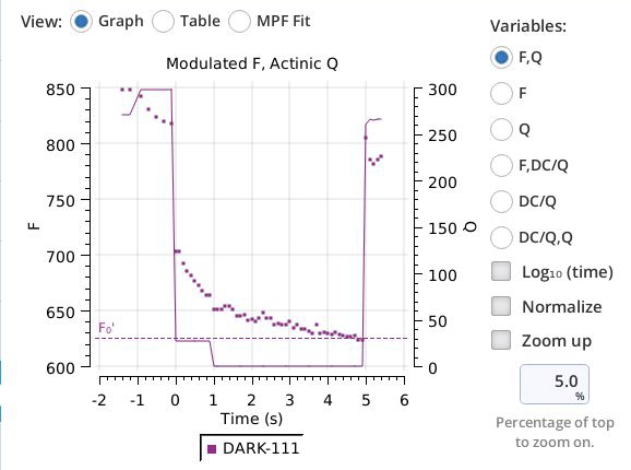
The default value of 5 seconds should be sufficient for most leaves. It should be long enough that fluorescence reaches minimum plateau. When NPQ relaxes, fluorescence yield increases. Fo’ is captured at the lowest fluorescence reading during the dark pulse. Better forward electron transport has been found when the far-red light is turned on a second before the actinic light is turned off, therefore set Before and After times accordingly.
Figure 8‑45. 5-second dark pulse. Fo' occurs at the 5 second mark so consider increasing the duration.
Margin
The purpose of the margin is to help visualize the dark pulse when looking at the data in the Results or Files tabs.


 :
:
 is computed, and used for the working value of Fʹo in computing quenching coefficients. If a dark pulse has been performed, its minimum value Fmin is recorded, and that is used for the working value of
  .
.