A Summary of a Multistage Data Processing Pipeline for the LI-710 and LI-720 Sensors on LI-COR Cloud
Author: Tyler Barker
Correspondence: envsupport@licor.com
Published: 8 December, 2025
Instruments: LI-710, Water Node, LI-720, Carbon Node, LI-COR Cloud
Keywords: flux gap filling, QA/QC, filtering, MDS gap filling, footprint modeling
Abstract
This document describes a technical approach to the data ingestion and processing pipeline designed for the data from the LI-710 Evapotranspiration Sensor and LI-720 Carbon Flux Sensor. The process combines preprocessing, quality control, and gapfilling techniques with available weather data to provide a continuous dataset.
1 | Introduction
The following process implements an end-to-end processing pipeline that inputs environmental sensor data, processes and merges the data, applies quality controls and diagnostic filters, gap-fills the dataset, and finally, prepares the data for modeling.
2 | Pipeline Overview
The pipeline is organized into several key steps. This overall workflow follows the structure of the FLUXNET2015 flux processing framework [1].
The term “removing” data here simply means that it will be removed from the cleaned dataset but will remain in the original cloud data-stream. Data processing only considers data from the current year:
- Data Scrubbing: Removes data based on metrics such as time division and length.
- Data Filtering: Removes data that are considered poor quality based on diagnostic issues, high frequency statistics, or are outside physically possible ranges.
- Preliminary Gap-Filling: Gaps in the data are preliminarily filled based on daily patterns to make a continuous signal for processing.
- Seasonal Decomposition: Data is modeled based on daily and seasonal patterns in a more robust way using Seasonal-Trend decomposition using LOESS (STL) modeling [2].
- Outlier Detection and Filtering: Employs robust scale estimators to identify and remove spikes based on earlier quality control methods [3].
- Turbulence Filtering: Calculates and performs turbulence threshold filtering on a daily or yearly basis depending on device type, data availability and sparsity [4].
- MDS Gap-Filling: Uses the marginal distribution sampling gap-filling approach (MDS) and external weather data to fill gaps in the cleaned data [5].
- Footprint Modeling: Model the flux footprint and daily footprint climatology for spatial flux processing.
- Data Storage: Saves data back to the cloud making it available in the dashboard.
3 | Methodology
3.1 | Data Scrubbing
This processing only considers datasets that are sampled at a 30-minute interval. Any dataset that is not sampled at a 30-minute interval starting from the first data point in a year will be removed from future processing. The dataset will also be required to have 10 days worth of data stored on the cloud to perform any cleaning and gap-filling processes. This equates to at least 480 30-minute data points. At least 2 months of data are required to perform USTAR threshold estimation. All data length requirements are based on the current year and will reset on the first day of the next year. Running the more robust, yearly processed USTAR filtering requires at least 10 days worth of data in each season, where a season is a period of 3 calendar months with the first season starting on the first of January at the location of the instrument and a total of four seasons. The details of the USTAR filtering approach will be explored later in this document.
3.2 | Data Filtering
The data is filtered into quality metrics based on instrument diagnostic and quality control tests.
3.2.1 | LI-710 Diagnostics Filtering
Some diagnostic codes represent a critical error in the measurement or processing of the 30-minute data. These codes for the LI-710 are as follows:
| Code | Description |
|---|---|
| 1 | Average flow for a 30-minute period is less than 125 sccm or greater than 330 sccm |
| 8 | Voltage is less than or equal to 1.6 volts for more than 50 % of time for a 30-minute period |
| 16 | Temperature is greater than 65 °C or less than −50 °C for more than 5 % of time for a 30-minute period |
| 128 | Poor sonic signals persist for more than 10% of time for a 30-minute period |
| 512 | High humidity shutdown |
| 1024 | Cold temperature shutdown |
If any of the above signals persist for more than 5 % of the high-frequency data in a single 30-minute time period, that flux value is assigned a quality flag of ‘medium’ (less than or equal to 15 %) or ‘low’ (greater than 15 %). Otherwise, the quality is considered ‘high’ (less than or equal to 5 %). These flags will be used in future processing stages.
3.2.2 | LI-710 QA/QC Filtering
The LI-710 ET values are directly filtered on the basis of physically possible values. The lower threshold of ET is −0.02 mm and an upper threshold is set at 0.8 mm in a 30-minute period. This removes any points that are beyond a realistic range and does not consider them in future steps.
3.2.3 | LI-720 Diagnostics Filtering
The diagnostic codes that signify some critical issue with the instrument’s measurements or processing for more than 10% of the 30-minute period in question for the LI-720 are as follows:
| Code | Description |
|---|---|
| 2048 | Relative signal strength is less than 80 % |
| 65536 | H2O concentration is out of range (< 10 or > 60 mmol/mol) |
| 131072 | CO2 concentration is out of range (< 0 or > 1500 μmol/mol) |
| 262144 | Sonic data frame is missing, no sonic data to analyze |
| 2097152 | More than 40 % of high frequency data is considered bad |
The data is then filtered on high frequency dataset statistics. The data is filtered based on the percentage of missing data in the sample count. If the percentage of missing data from this sample count are between 5 and 15 %, the quality of this data point is set to a quality flag of ‘medium’ and if the percentage is above 15 % the quality flag is set to ‘low’. Any other percentage is considered ‘high’. The ‘low’ quality data will be removed from future processing steps and only ‘medium’ quality data will be considered for outlier detection filtering. ‘high’ quality data is used as modeling data for outlier detection, but it is not removed if flagged. The data quality control structure follows [6].
3.2.4 | LI-720 QA/QC Filtering
The LI-720 flux values are directly filtered on the basis of plausible values. The lower threshold of CO2 flux is −100 μmol m−2 s−1 and an upper threshold is set at 50 μmol m−2 s−1. This removes any points that are beyond a realistic range and does not consider them for future steps.
The data is then filtered on the quality of the CO2 concentration and vertical wind speed signal qualities. This is measured by the percentage of missing data in the CO2_RECORDS and W_RECORDS. If the percentage of missing data from either of these signals are between 5 % and 15 %, the quality of this 30 minute average data point is set to a quality flag of ‘medium’ quality and if the percentage is above 15 % the quality flag is set to ‘low’ quality. The ‘low’ quality data will be removed from future processing steps and only ‘medium’ quality data will be considered for outlier detection filtering whereas ‘high’ quality data is only used as modeling data for outlier detection.
The relative signal strength indicator (RSSI) is also used as a quality-control parameter for the LI-720 measurements. Data are classified into three quality levels based on the percentage of valid signal detected during each 30-minute averaging period: measurements with RSSI greater than 95 % are assigned a ‘high’ quality flag, those between 90 % and 95 % are considered ‘medium’ quality, and values below 90 % are labeled ‘low’ quality.
The LI-720 calculates more high frequency statistics that can be used for quality flagging. Specifically, the (3), (4) and (5) “Source of error” repeated here directly from [6] (Table 1):
Once all data quality checks are performed, 'low' quality data is removed, and all other data is passed to the next step.
3.3 | Turbulence Filtering
Turbulence (USTAR) filtering is applied differently for the LI-710 and LI-720 instruments due to differences in available variables and sensor design.
3.3.1 | LI-710 Turbulence Measure
For the LI-710, which does not provide direct measurements of the friction velocity (u∗), the standard u∗-based turbulence filter is approximated using the standard deviation of the vertical wind speed (σw) as a proxy. Low σw values indicate insufficient turbulence and a higher likelihood of flux underestimation under stable conditions. Flux records with σw below a defined threshold are therefore removed, effectively excluding periods of near-still air when turbulent exchange is weak.
3.3.2 | LI-720 Turbulence Measure
For the LI-720, a more sophisticated, dynamic turbulence filtering procedure is applied. Each day, a change-point detection algorithm determines the daily u∗ threshold by fitting two linear regressions to the relationship between the measured flux and u∗. One regression is unconstrained, while the other is forced through the origin. The intersection of these two lines defines the daily u∗ threshold, below which data are excluded as low-turbulence conditions.
At the end of each year, the dataset is further divided into four seasonal subsets. For each season, 100 bootstrap samples (random draws with replacement) are generated, and both the change-point detection and moving-point u∗ filtering methods are applied [4, 5]. Each filtered dataset is subsequently gap-filled (procedure described below). The mean of all realizations is then taken as the final, seasonally adjusted flux estimate. This combined approach ensures that the turbulence filtering is both statistically robust and sensitive to seasonal changes in canopy structure and atmospheric stability.
3.4 | Preliminary Gap-Filling
The data at this stage have some gaps that exist due to the previous data quality filtering and environmental or physical instrument issues such as power outages. In order for the daily and yearly cycles to be modeled in the data for further analysis, a preliminary gapfilling on the CO2 flux (LI-720) and the ET measurements (LI-710) must be performed. This transforms the measurement data into a continuous time series and is done by modeling the data based on time of day (an STL model) and fitting new data using the K-nearest neighbors approach [7]. This more simplistic technique will relate the flux values of previous cycles (days) to the current day in order to create a first approximation of the missing data. This imputed data is omitted after the de-spiking process is performed.
3.5 | Outlier Detection and Filtering
This workflow follows the procedure described in [6, 8] and originally implemented in the RFlux project. It has been reimplemented here with minor modifications to run in a different environment.
-
Step 1: Applies STL LOESS decomposition to a time continuous dataset to achieve a best fit model accounting for diurnal and seasonal patterns.
-
Step 2: Finds the residuals (observed - modeled) and bins them into 10 groups equally spaced in the magnitude of the modeled flux value.
-
Step 3: Detects outliers through a Laplace distribution thresholding using robust scale estimators such as the median absolute deviation (MAD).
-
Step 4: Generates a complete timestamp range and merges it with the original dataset, flagging the missing values.
Once these outliers are found, the data that was flagged as ‘medium’ quality and an outlier is removed for the LI-720. All data that is flagged as ‘high’ quality is not removed even if it is also flagged as an outlier.
Due to a lack of high frequency statistics in processing, an aggressive approach is adopted. Any data that are flagged as an outlier in this process are removed.
3.6 | Weather Data Imputation
To enhance the accuracy of gap-filling and support downstream modeling, the pipeline begins by retrieving relevant weather data. This involves querying the OpenMeteo API, an opensource weather API service for modeled key environmental variables including temperature, VPD, and shortwave radiation [9].
Once retrieved, the hourly weather data is resampled to match the sensor data’s 30-minute resolution using linear interpolation. This ensures temporal alignment with the flux measurements and provides a continuous weather context for imputation and modeling. A linear regression is performed for each variable recorded by the LI-710 or LI-720 between the observed and modeled values.
The modeled data are then corrected by applying the inverse regression, using the observed measurements as the baseline. This adjustment is necessary because, while the modeled data typically capture the relative variations in the observations, their absolute magnitudes often differ. If a variable is not directly measured by the instrument, the unadjusted modeled output is used instead.
3.7 | MDS Gapfilling
After sensor and weather data have been scrubbed, filtered, preliminarily gap-filled, and despiked the dataset is prepared for data imputation. The data is processed by the Marginal Distribution Sampling (MDS) algorithm that uses like data from recent and near-future measurements in temperature, Vapor-pressure deficit (VPD), and solar radiation to impute the data [5]. This creates a continuous set of flux data that can be used for future processing such as flux accumulation, forecasting, and spatial extrapolation.
3.8 | Data Storage
3.8.1 | Cleaned and Gap-filled Data
The processing pipeline runs each day and considers all the data in each timeseries from the beginning of the year. Only the data from the last day is written back to the cloud. Therefore, cleaned data and gap-filled data will not change, on a daily basis, for days in the past but could ideally change given all available data. This approach is used to maintain a semi-static dataset for quick analysis throughout the year, but also utilize all available data for a best estimate at the most recent flux data.
To maintain a best-estimate process on longer time periods, cleaned and gap-filled data streams are recalculated and saved on a monthly and yearly basis. This will overwrite the data for the last month or year, respectively. This means that at the end of a calendar year, this data processing will use all available data in that year. At this point the data-stream will remain static.

3.9 | Footprint Data
For the daily footprint climatology of the LI-720 system, the two-dimensional flux footprint parameterization developed by Kljun et al. (2015) [10] is applied. This model estimates the upwind source area contributing to the measured fluxes at the sensor height by incorporating boundary-layer characteristics, surface roughness, wind speed, wind direction, and atmospheric stability. The footprint is computed for each 30-minute period of the day corresponding to the flux measurements and then aggregated to generate a single daily footprint climatology.
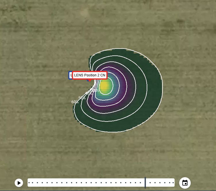
In this implementation, key meteorological and turbulence parameters are derived from both the instrument and external data sources. u∗ for the LI-710 is estimated using the standard deviation of the vertical wind component (σw) as a proxy for turbulence intensity. Additional inputs, including wind speed and wind direction, are obtained from the Open-Meteo API.
4 | References
| 1 | Pastorello, G., Trotta, C., Canfora, E. et al. (2020)The FLUXNET2015 dataset and the ONEFlux processing pipeline for eddy covariance data. Scientific Data 7, 225. https://doi.org/10.1038/s41597-020-0534-3. |
| 2 | Cleveland, R.B., Cleveland, W.S., McRae, J.E., Terpenning, I. (1990). Stl: A seasonal-trend decomposition procedure based on loess. Journal of Official Statistics; Statistics Sweden, 6(1):3–73. |
| 3 | Rousseeuw, P. J., and Croux, C. (1993). Alternatives to the Median Absolute Deviation. Journal of the American Statistical Association, 88(424), 1273–1283. https://doi.org/10.1080/01621459.1993.10476408. |
| 4 | Papale, D., Reichstein, M., Aubinet, M., Canfora, E., Bernhofer, C., Kutsch, W., Longdoz, B., Rambal, S., Valentini, R., Vesala, T., and Yakir, D. (2006) Towards a standardized processing of Net Ecosystem Exchange measured with eddy covariance technique: algorithms and uncertainty estimation, Biogeosciences, 3, 571–583, https://doi.org/10.5194/bg-3-571-2006. |
| 5 | Reichstein, M., Falge, E., Baldocchi, D., Papale, D., Aubinet, M., Berbigier, P., Bernhofer, C., Buchmann, N., Gilmanov, T., Granier, A. and Grünwald, T. (2005). On the separation of net ecosystem exchange into assimilation and ecosystem respiration: review and improved algorithm. Global change biology, 11(9), pp.1424-1439. https://doi.org/10.1111/j.1365-2486.2005.001002.x |
| 6 | Vitale, D., Fratini, G., Bilancia, M., Nicolini, G., Sabbatini, S., and Papale, D. (2020) A robust data cleaning procedure for eddy covariance flux measurements, Biogeosciences, 17, 1367–1391, https://doi.org/10.5194/bg-17-1367-2020. |
| 7 | Cover, T. and Hart, P. (1967) Nearest neighbor pattern classification. IEEE Transactions on Information Theory, 13(1):21–27. |
| 8 | Vitale, D., Papale, D., and ICOS-ETC Team. (2021) RFlux: An R Package for Processing and Cleaning Eddy Covariance Flux Measurements. ICOS Ecosystem Thematic Centre (ICOS-ETC), Viterbo, Italy. R package version 3.2.0, available at https://github.com/icos-etc/RFlux. |
| 9 | Open-Meteo. Open-meteo free weather api, n.d. https://open-meteo.com. |
| 10 | Kljun, N., Calanca, P., Rotach, M.W. and Schmid, H.P. (2015). A simple two-dimensional parameterisation for Flux Footprint Prediction (FFP). Geoscientific Model Development, 8(11), pp.3695-3713. https://doi.org/10.5194/gmd-8-3695-2015. |