


Using the LI-600F or LI-600N red LEDs as a variable actinic light source
Authors: S.D. Loriaux and D. Lynch
Correspondence: envsupport@licor.com
Published: 01 November 2026
Instruments: LI-600, LI-600N, LI-6800
Keywords: porometry, steady-state ETR-Q curves, PPFD
Abstract
This application note describes how the LI-600F/N red LEDs can be controlled as a variable actinic light source for steady-state and rapid electron transport rate–irradiance (ETR–Q) curves. It presents the required hardware, LED-frequency commands, calibration, dark cover, and both manual and Python-based workflows. A general calibration supports approximately 0 to 2,000 µmol m−2 s−1 with typical error of ±10%. LI-600 and LI-6800 steady-state ETR responses were similar at or below ambient irradiance, but LI-600 values were lower above ambient. Rapid curves produced lower ETR and stomatal conductance than steady-state curves and should be interpreted as transient, light-history-dependent measurements rather than substitutes for steady-state curves.
1 | Introduction
Electron transport rate (ETR) is derived from chlorophyll a fluorescence measurements:
1ETR = ΦPSII × PPFD × ɑ × 0.5
The parameters ΦPSII and PPFD are measured by the LI-600F/N, while ɑ is the leaf absorptance (typically 0.84 for sunlight) and 0.5 is the ratio of light absorbed by PSII vs PSI. ETR provides a rapid and sensitive functional measurement of the light reactions of photosynthesis (Genty et al., 1989). ETR provides information on the efficiency and capacity of the photosynthetic electron transport chain and can be used to characterize photosynthetic responses to irradiance similarly to A–Q curves. Steady-state and rapid ETR–Q curves have been employed to assess photosynthetic capacity, light-use efficiency, and photoprotective responses (de la Fuente et al., 2023; Rascher et al., 2000).
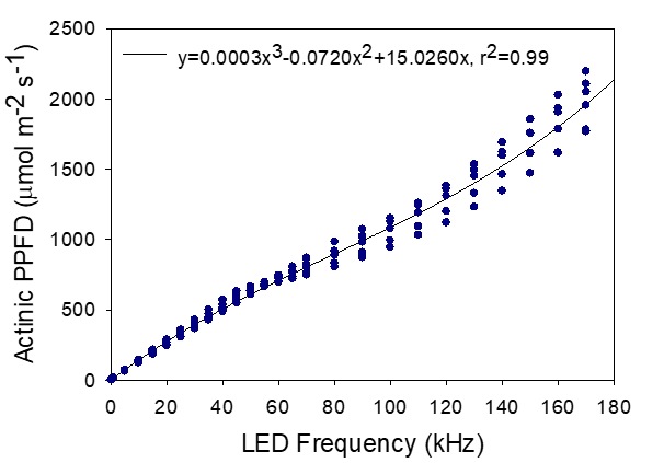
The LI-600F and LI-600N are portable instruments designed for rapid measurements of stomatal conductance (gsw) and chlorophyll a fluorescence under ambient field conditions. The LI-600F/N red LEDs normally used for modulated and saturating illumination can also provide variable actinic light when the pulse frequency is controlled. The actinic LED output as a function of frequency setpoint was calibrated in an integrating sphere using a spectroradiometer for multiple LI-600F instruments. Figure 1 shows the results and the best-fit non-linear calibration function.
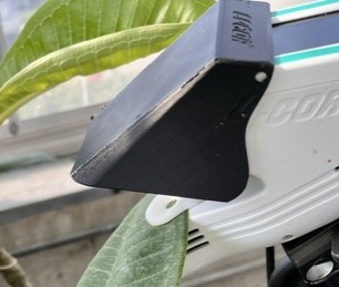
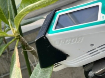
For many situations, the ambient light should be excluded using a custom dark cover (see Dark cover (optional)) so that LED output, rather than the external environment, defines the actinic treatment. In addition, this cover can help facilitate dark-adapted fluorescence measurements with the instrument.
2 | Materials
The materials used in this document include a USB-to-UART cable, a dark cover, LI-600 software, and either a terminal program or Python with Spyder.
| Description | Part # |
|---|---|
| USB-to-UART adapter cable | 9900-053 |
| Dark Cover (see Appendix A) | n/a |
2.1 | Installing the USB-to-UART cable
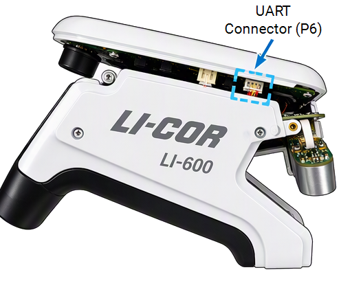
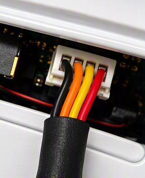
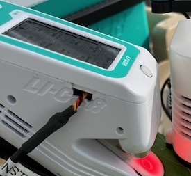
Remove the outer LI-600 case to access the fluorometer control connector. You can also purchase an extra case half to be able to add a slot to provide access to this connector when the case is installed.
2.2 | Dark cover (optional)
An ambient light exclusion or dark cover is optional, but highly recommended. It is a custom 3D-printed cover that masks the chamber and the LI-600 quantum sensor while allowing the leaf to extend from the chamber edges. You can print your own using the CAD file linked in Appendix A.
2.3 | Software control
Use the LI-600 software to create configurations and retrieve final instrument data. Access to LED frequency control is not currently available in the LI-600 interface. To control the fluorometer’s LEDs, use one of the options described in Option A: Serial terminal software or Option B: Python / Spyder.
To identify the COM port that hosts the USB-to-UART cable, connect the USB-to-UART adapter to the computer and open Windows Device Manager. Expand Ports (COM & LPT) and identify the USB serial device. Note the COM port number shown in parentheses (for example, COM4). Use this COM port when establishing the serial connection to the LI-600. If multiple USB serial devices are listed, unplug and reconnect the adapter to determine which COM port corresponds to the cable.
2.4 | Option A: Serial terminal software
Use serial terminal interface software such as Tera Term, PuTTY, or RealTerm.
-
Best used for one-off command testing and manual stepping.
-
Select the correct COM port, and close other programs that may already have the port open.
-
Configure the serial connection as 115200 baud, 8 data bits, no parity, 1 stop bit, and no flow control.
-
Set the terminal to transmit a line feed / ASCII newline (0x0A) at the end of each command. Incorrectly terminated commands are ignored.
2.5 | Option B: Python / Spyder
Use Python 3 with the pyserial package.
-
Spyder can be used as the development environment, but the script is not dependent on Spyder. Python is best used for repeatable light sequences, timed holds, automatic logging, and recording actual command history.
-
Select the correct COM port, and close other programs that may already have the port open.
-
Open the serial port at 115200 baud, 8-N-1, set the pulse-frequency, and then manually log a value on the instrument or have the program trigger the instrument’s log function.
2.6 | Command syntax and serial behavior
Commands are plain-text strings sent to the P6 debug UART. Every command must end with ASCII newline (0x0A). Use frequency values in Hz (the general actinic calibration function in Figure 1 is shown in kHz).
The command to set the LED frequency is set -pulse_freq <frequency_in_Hz>. The frequency range is from 10 to 7,500,000 Hz.
Example:
set -pulse_freq 50000The calibration frequency-to-PPFD conversion function is
2Actinic PPFD = 3.0 × 10−13x3 − 7.20 × 10−8x2 + 0.015026x
The typical error is ±10% across the 0 to 2,000 µmol m−2 s−1 range using this general calibration function. This calibration was measured in an integrating sphere with a spectroradiometer using multiple LI-600F instruments.
3 | Example: Manual steady-state ETR–Q curve
Begin with a light-adapted leaf and measure the fluorescence light response after allowing the leaf to approach a stable response at each actinic level.
-
Configure the instrument using the LI-600 interface software:
-
General: Use Fluorometer and if measuring outside, Use GPS and Leaf Angle
-
Data Labels: Do not use Prompt On Log. Optionally, set Data Labels to log manually at the beginning of the curve.
-
Automode Setup: Do not use Automode. Set desired stability criteria to Medium or Custom.
-
Remarks: No changes.
-
Measurement Settings: No changes (verify default settings are Multiphase Flash: Intensity of 7000, Phase 1 to 3 lengths of 300 ms, and ramp of 25%).
-
Display Layout: No changes
-
Warm up the LI-600 for 15 minutes in the environment in which you will be taking measurements. If using GPS, ensure the map pin is displayed.
-
-
Select the configuration made earlier.
Follow the instructions regarding matching. Then, verify normal RH, temperature, and flow values are displayed.
-
Connect the LI-600 USB-to-UART control cable to your computer, identify the COM port and open the terminal or Python script.
-
(Optional) Install the dark cover and verify that it does not interfere with chamber closure or leaf placement.
-
Verify the lowest and highest intended light settings before placing a leaf in the chamber.
-
Document the leaf’s ambient light before enclosure and whether the initial chamber intensity was above ambient. Place the leaf in the chamber, install the dark cover, and begin at the highest planned actinic level and set the frequency using the terminal software or Python.1
-
Allow the leaf to light-adapt until the selected physiological variables are stable.
-
-
Log the first point, then step downward through the planned light sequence.
-
Wait at each light level for 3 to 5 minutes until stable and then log a data point.
At each level, record the commanded frequency and calculated PPFD.
-
After the final point, turn the actinic LEDs off, remove the cover, and verify the instrument returns to normal operation.
4 | Example: Automated steady-state ETR–Q curve
4.1 | Objective
This example has the same objective as the example above, but uses Python code to automatically change the light level, wait a period, log data, and move to the next light level.
Download the Python code here:
Automated stead-state ETR-Q curve Python code: licor.app.boxenterprise.net/s/5iejprsevhfavrmg9ysdkuk89uuh18f0
-
Follow steps 1 to 5 above, except run the example curve in the Python script.
-
When the program starts:
-
You will first be asked for the actinic light levels in the order they should be used:
LI-600 Fluorescence Light-Response Curve
==================================
Enter the COM port assigned to the LI-600 USB-to-UART cable (for example, COM9): COM6
Enter the Qact values for the light-response curve.
Valid range: 0 to 2100 umol m-2 s-1
Enter the values in the order they should be run.
Example: 2100, 1900, 1500, 1000, 700, 400, 200, 100, 0
-
You will be asked for the wait time to use between light levels:
Enter the wait time at each Qact level, in seconds:
-
Next, you will select whether to use a general calibration or custom calibration:
Select the LED calibration:
1 = General calibration
2 = Custom calibration
Enter 1 or 2: 1
-
Then, the light response curve will begin and will report when it is done:
Using the general calibration:
Qact = 3.0e-13*f^3 - 7.2e-8*f^2 + 0.015026*f
Frequency f is in Hz.
Valid Qact range: 0 to 2100 umol m-2 s-1
Calibration: General calibration
Planned light-response curve:
1. Qact = 2000.0 umol m-2 s-1 -> 173121 Hz
.
.
.
==========================================
Point 1 of x
Requested Qact: 2000.0 umol m-2 s-1
LED frequency: 173121 Hz
Calibration-predicted Qact: 1999.99 umol m-2 s-1
Light level set. Waiting 300.0 seconds...
Logging point...
Point 1 logged.
==========================================
.
.
.
Done:
-
-
After the final point, turn the actinic LEDs off, remove the cover, and verify the instrument returns to normal operation.
4.2 | Example data
Example steady-state ETR-Q curves measured on greenhouse-grown sunflower, soybean, and corn during winter.
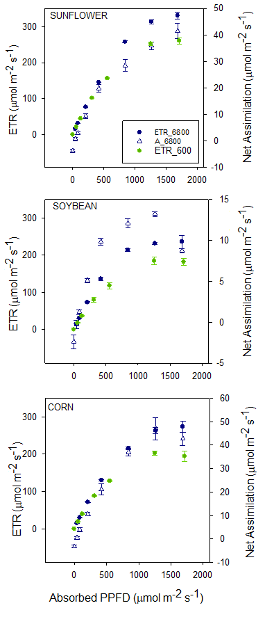
Steady-state light response curves were measured on the same greenhouse-grown sunflower, soybean, and corn leaves using the LI-600F and LI-6800F. Leaves were first light-adapted in the chamber at the highest light level until A and gsw were stable, then light was decreased for 5 min at each step. The LI-6800 was set for 90% red and 10% blue. At light levels equal or below ambient, no significant differences were found in the ETR-Q curves between instruments. However, at light levels above ambient (~500 µmol m−2 s−1 ave. ambient PPFD), the LI-600 ETR values were lower, likely due to light-adapting with 100% red in the LI-600 versus red and blue in the LI-6800, as well as lack of other environmental controls in the LI-600.
5 | Example: Rapid / Instant ETR–Q curve
5.1 | Objective
Provide a short-duration screening curve that intentionally samples transient rather than steady-state responses.
-
Begin by preconditioning the leaf and follow steps 1 to 4 under the manual curve above.
-
Begin at the lowest planned actinic level and run the same automated curve above.
-
Enter the Qact values, stepping upward from low to high light.
-
Wait time at each light level is only 30 seconds.
-
Select the general or custom calibration.
-
Continue through the complete predefined sequence without changing leaf position or cover placement.
-
-
After the final point, turn the actinic LEDs off, remove the cover, and verify the instrument returns to normal operation.
5.2 | Example data
Rapid or “instant” fluorescence light-response curves are collected before photosynthesis reaches steady state at each irradiance and should therefore be validated against measurements made under steady-state conditions.
One approach is to compare effective PSII quantum yield measured during the rapid curve with measurements obtained under ambient conditions when photosynthesis is at steady state. If the two responses agree over the physiologically relevant irradiance range, the rapid-curve measurements may be interpreted directly. If they differ by a relatively constant offset, an appropriate correction may be possible.
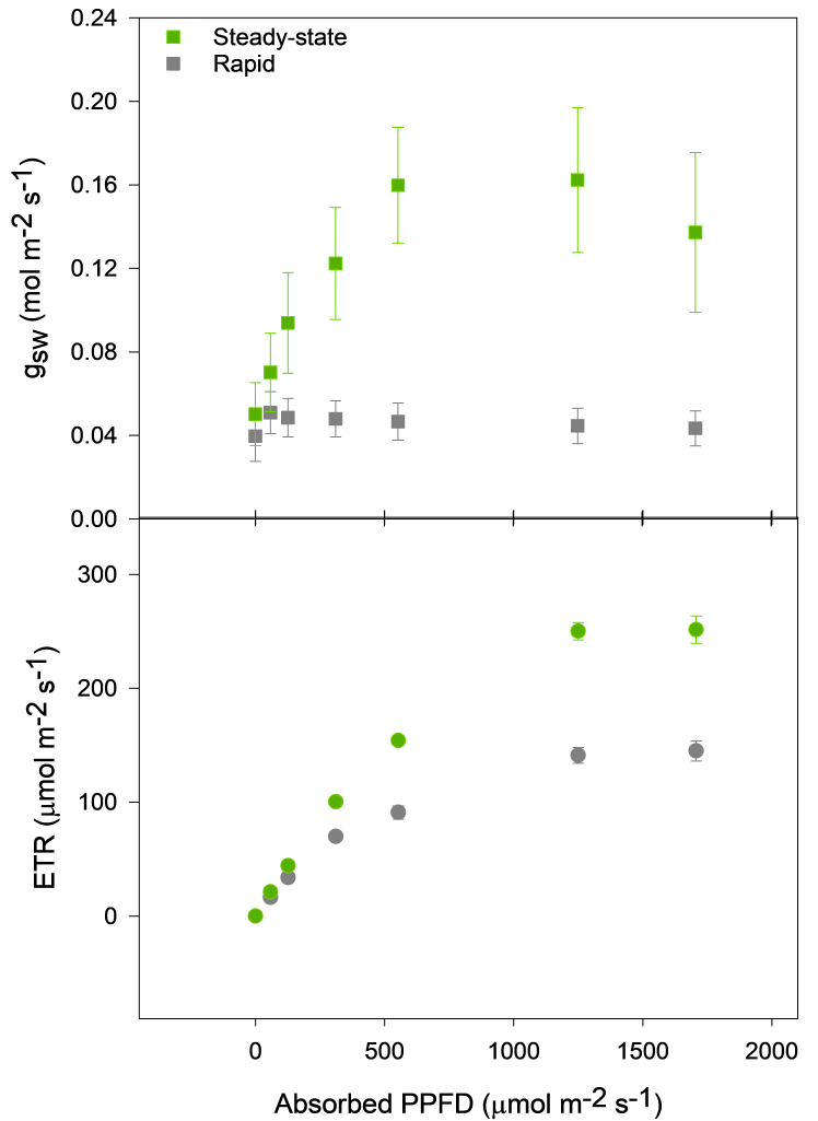
In this study, steady-state and rapid ETR-Q curves were compared using greenhouse-grown sunflower leaves. For the steady-state curves, leaves were first adapted to high light, and irradiance was then decreased in 5-min steps. Rapid curves followed the ascending “instant” light-response approach, with irradiance increasing from low to high at 30-s intervals. The rapid curves produced consistently lower ETR, and generally lower stomatal conductance (gsw), than the steady-state curves. These results demonstrate that measurements obtained during a rapid curve are not necessarily equivalent to steady-state measurements and can retain effects of the leaf's recent light history and its transient physiological response to changing irradiance. Rapid ETR-Q curves are best interpreted as a standardized measure of the dynamic photosynthetic light response rather than as a direct substitute for a steady-state ETR-Q curve. Where quantitative estimates of steady-state behavior are desired, the rapid-curve protocol should first be compared with steady-state measurements over the relevant irradiance range.
6 | Conclusions
The LI-600F/N hardware can be used to generate variable pulsed red actinic light and collect both steady-state and rapid ETR–Q curves. Rapid curves systematically differ from steady-state curves and should be reported as a distinct measurement protocol. The custom dark cover is a useful accessory for constraining actinic control as well as facilitating dark-adapted measurements.
7 | Appendix A
The linked file is a 3D model of the dark cover that can be printed on a 3D printer.
Dark cover 3D model: licor.app.boxenterprise.net/s/g4aq3a116cio6s964f9t31znm1yirb37.
8 | References
Genty, B., Briantais, J., & Baker, N. R. (1989). The relationship between the quantum yield of photosynthetic electron transport and quenching of chlorophyll fluorescence. Biochimica et Biophysica Acta (BBA) - General Subjects, 990(1), 87-92. https://doi.org/10.1016/s0304-4165(89)80016-9
Martos de la Fuente, G. C., Viñegla, B., Illana Rico, E., & Fernández Ocaña, A. M. (2023). Study of the photosynthesis response during the gradual lack of water for 14 Olea europaea L. subsp europaea cultivars and their adaptation to climate change. Plants, 12(24), 4136. https://doi.org/10.3390/plants12244136
Rascher, U., Liebig, M., & Lüttge, U. (2000). Evaluation of instant light‐response curves of chlorophyll fluorescence parameters obtained with a portable chlorophyll fluorometer on site in the field. Plant, Cell & Environment, 23(12), 1397-1405. https://doi.org/10.1046/j.1365-3040.2000.00650.x