In this chapter we provide information about using the instrument in field or laboratory applications. We cover connecting plumbing to the air inlet, retrieving data, and other applications.
Flow schematic
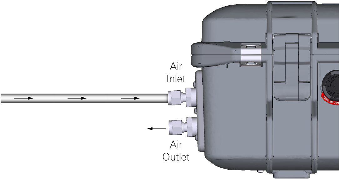
During normal operation, air is drawn into the analyzer through the air inlet (Figure 3‑1). Air flows through the optical bench and phase adjuster and is exhausted through the air outlet. In the optical bench, the pressure is drawn down to about 40 kPa. When the instrument is powering down, air is circulated in a closed loop through the desiccant to ensure that air remaining in the system is free of moisture, preventing condensation when the instrument is powered off.

Regularly check the H₂ measurement and adjust the soft zero
To measure H2 in air, the H2 zero should be set regularly using the Soft Zero procedure. This procedure adjusts the hydrogen-only values to correct for offsets that can be introduced by instrument drift or shifts in the position and orientation of the instrument. For the most dependable H2 measurements, avoid dramatic changes in temperature, position, and orientation during a measurement, and initiate the soft zero as often as needed.
What is the soft zero?
Soft zero applies a simple offset to the reported hydrogen-only concentrations to ensure the instrument reports zero H2 when the sample is free of hydrogen gas. In many cases, atmospheric air is effectively H2-free (~500 ppb) and can be used as a soft zero reference gas. No adjustments to the measurement of CH4 or H2O are made during the soft zero procedure.
Conversely, the zero calibration procedure (see Setting the H₂, CH₄, and H₂O zeros) adjusts all reported species including H2, CH4, and H2O. This requires that none of the reported species are present in the sample. Atmospheric air contains significant concentrations of H2O (~20,000 ppm) and CH4 (~2 ppm), and special gas mixtures must be used for the full zero procedure (see Instrument calibration).
When to adjust the soft zero?
The soft zero can be initiated by the instrument operator through the interface or command line. With practice, you'll get a better sense of when the adjustment is needed, but in general, follow these guidelines to determine when to adjust the soft zero:
-
After powering on the instrument, allowing it to warm up for one hour, the H2 measurement has stabilized, and at least once per day after that. Do not set the soft zero if the H2 measurement is unstable.
-
If the reported H2 value is negative or not within 15 ppm of 0 (zero) even though there is no source of H2 present.
-
If there are dramatic changes in the relative concentrations of gases in the air.
-
If environmental conditions have changed, such as movement from indoor to outdoor temperatures or after exposure to solar load.
-
After moving or changing the orientation of the instrument.
How to adjust the soft zero?
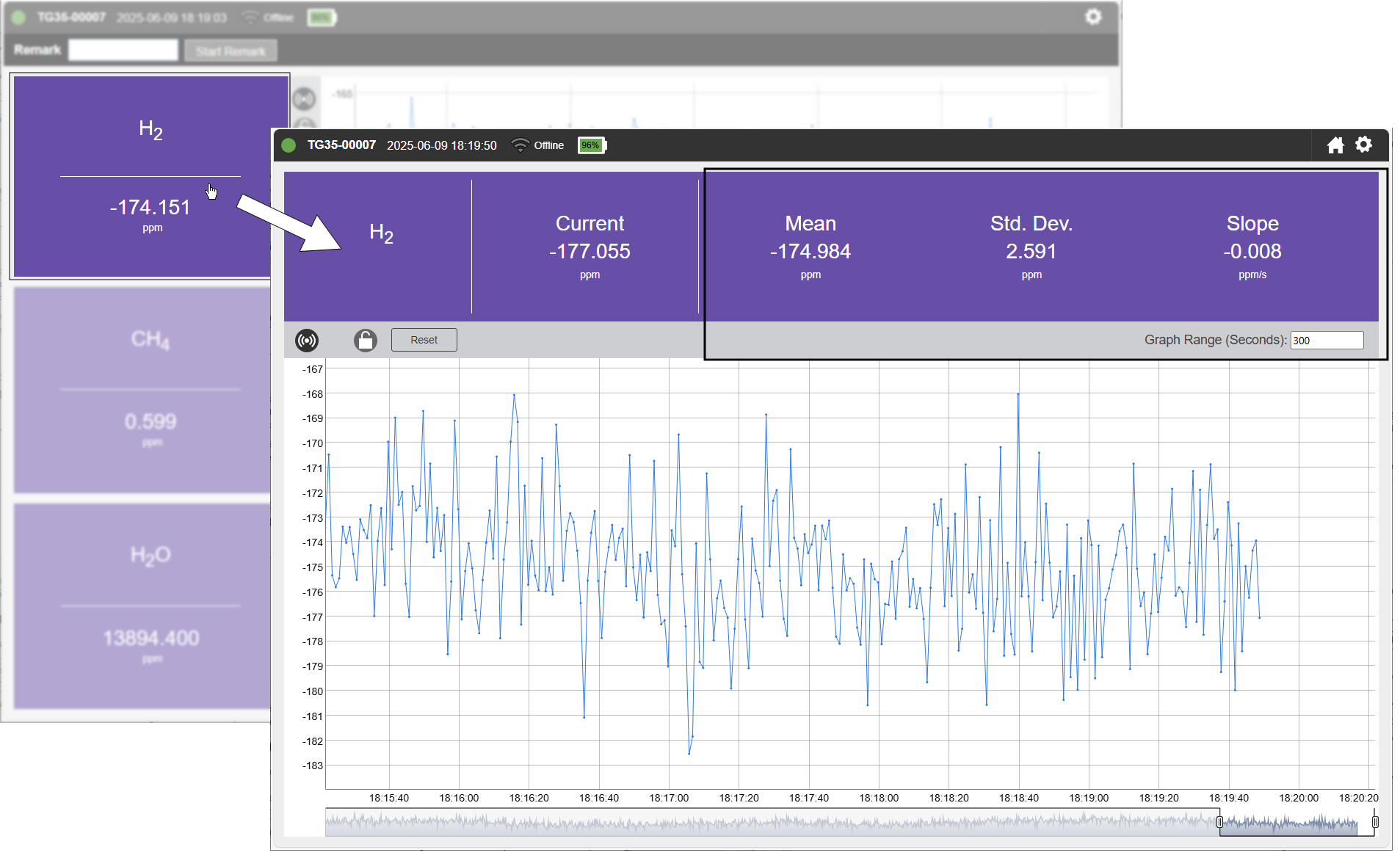
In ambient atmospheric air, H2 concentrations are typically very close to zero (500 ppb) unless there is a source of H2. Sources of environmental H2 include coal fields, leaky natural gas sources, and wetlands with high levels of anaerobic decomposition, to name a few. If you are certain that there is no environmental source of H2, you can set the soft zero in ambient air. If, however, ambient air has non-zero H2, use a tank of hydrogen-free air instead. Connect the tank to the inlet as described in Connecting the air inlet and outlet. Allow the measurement to stabilize, as indicated by the slope and standard deviation (see Figure 3‑2). The slope should be near zero. Do not adjust the soft zero if the measurement is not stable.
Under Calibrations > Zero H2 Only, click Zero H2 (see Figure 3‑3).
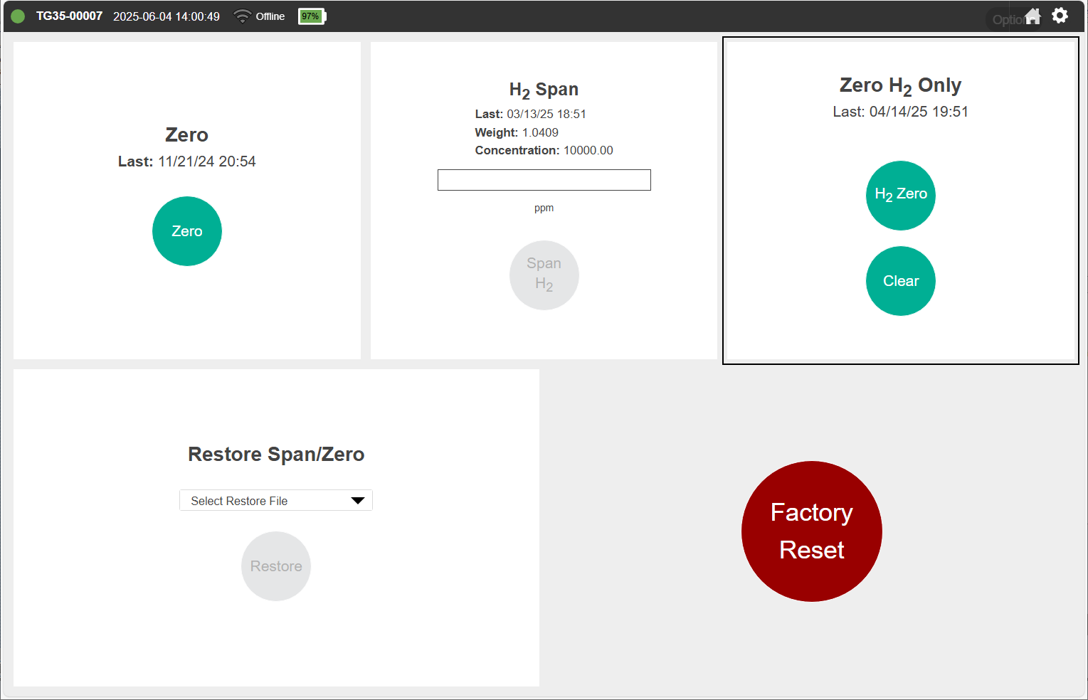
Observe the measurement after adjusting the zero to be sure the changes had the desired effect. If something is amiss, click Clear to discard the changes.
Connecting the air inlet and outlet
Air is drawn into the sample cell through the air inlet. Connect tubing to the inlet with the nut, bushing, and ferrule from the accessories kit. Optional stainless steel inserts (300-18126) are included for use with soft tubing. Tubing can be connected to the inlet and the outlet in the same way.
Caution: Be careful when working near standing water. If water is drawn into the air inlet, the instrument will have to be repaired at the factory.
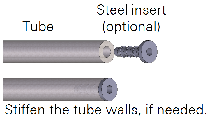
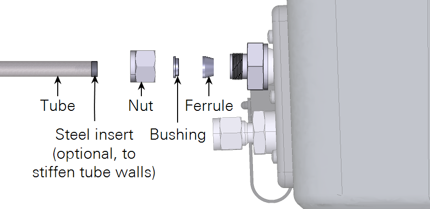
To connect a ¼" outside-diameter metal or plastic tube to the compression fitting, insert the nut, bushing, and ferrule over the tube. Then tighten the nut over the ferrule until it is finger tight. Tighten it an additional 1-¼ revolutions if you are connecting the tube for the first time. For highly pliable plastic tubing, place a stainless steel tube insert (300-18126) inside the tubing to make it rigid enough.
When reconnecting a plastic or metal tube that has been connected previously, simply tighten it ¼ turn beyond finger tight.
Caution: Abrupt pressure transients up to 35 kPa above or below ambient pressure may cause momentary status warnings, inlet plugged warnings, and measurement inaccuracies. Longer lasting pressure excursions or larger pressure transients may cause the instrument to reinitialize measurement control loops.
Plumbing a subsample
A typical sampling application will use the LI-7835 to subsample a gas from a main sample line. Air passes a single time through the gas analyzer before it is discharged. Air supplied to the sample inlet should be between ambient and 35 kPa (5 PSI) above ambient.
Retrieving data from the instrument
The LI-7835 records all of its data after it has warmed up. There is no way to turn data logging on or off because data are always logged. The instrument supports two protocols for transferring data:
- Direct download using TCP/IP (internet protocols; see Downloading a data file) and
- MQTT (Message Queuing Telemetry Transport; see Communication with the MQTT protocol).
Downloading a data file
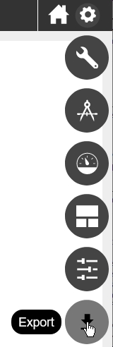
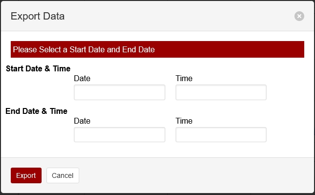
To retrieve data from the instrument, click Options > Export. Specify a date range and time period. Dates are displayed as YYYY-MM-DD. Time options are given in a 24-hour clock (00:00 through 24:00). Click Export. The web browser will prompt you to save or open the file, and then provide a text file with the requested data. The file has a .data extension. Measurements are recorded as tab-delimited text that can be opened in a text editor or spreadsheet application.
Components of the data file
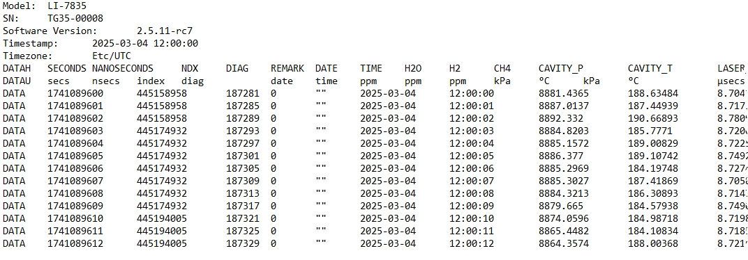
The text file will include a file header, data header, and data.
File header
The file header provides information about the instrument that measured the data.
Data header
The data header identifies the columns of values that are in the file. You'll see two rows: one called DATAH, which gives the variable names for the corresponding columns, and one called DATAU, which gives the units for the corresponding columns.
| DATAH | DATAU | Description |
|---|---|---|
| SECONDS | secs | Seconds past the universal epoch (Unix time). |
| NANOSECONDS | nsecs | Nanoseconds of the seconds |
| NDX | index | A count of scans. At four scans per second, the value increases by four counts per second. |
| DIAG | diag | Diagnostic code (see Status codes) |
| REMARK | - | The remark entered in the Remark field |
| DATE | date | Date of the record in yyyy-mm-dd |
| TIME | time | Time of the record in HH:MM:SS (according to the instrument clock) |
| H2O | ppm | Water vapor mol fraction |
| H2 | ppm | H2 mol fraction in dry air |
| CH4 | ppm | CH4 mol fraction in dry air |
| CAVITY_P | kPa | Optical cavity pressure (typically near 39) |
| CAVITY_T | °C | Optical cavity temperature (typically near 55) |
| LASER_PHASE_P | kPa | Laser phase pressure |
| LASER_T | °C | Laser temperature |
| RESIDUAL | n/a | Difference between raw and best fit spectra |
| RING_DOWN_TIME | µsecs | Indicator of cavity resonance |
| THERMAL_ENCLOSURE_T | °C | Optical enclosure temperature |
| PHASE_ERROR | counts | Dimensionless indicator of mode lock state |
| LASER_T_SHIFT | °C | Shift in laser center wavelength from factory calibration |
| INPUT_VOLTAGE | V | Power supply voltage |
| CHK | CHK | Checksum; to ensure that the receiving software received the data without error, and to reject corrupted data lines |
Time, data , and diagnostics
The time, data, diagnostics, and remark are given under the header.
The relationship between Unix Epoch time and the time stamp
The instrument measures time based upon the number of seconds past the Unix epoch (GMT: Thursday, January 1, 1970 12:00:00 AM). This value is represented in the Seconds column of the data set. You can easily convert the Unix epoch to date and time using online resources (e.g., https://www.epochconverter.com). If you have selected a time zone, the Date and Time columns will represent the Unix epoch time adjusted by an offset for the time zone.