Calibration Issues
The LCF's Light Sensor
The LCF has independently controlled red and blue LEDs for actinic light to drive photosynthesis. There are also two red LEDs for measuring fluorescence, and a far red LED for driving PS I. The internal light sensor in the LCF sees - directly or indirectly - all of these LEDs. The factory calibration of this sensor to the actinic LEDs consists of generating two factors (one for red, one for blue) that relate actual light output to sensor signal. Actual light output is measured with an integrating sphere and an LI-1800 Spectroradiometer. No calibration factor is generated for the measuring beam, or for the far red LED.
The far red LED has a definite impact on the internal light sensor. Typically, a setting of 10 on the far red LED (and all other LEDs off) will cause the light sensor to read 30 or more. However, the actual quantum flux is usually about 10 μmol m-2 s-1 at a setting of 10, so don’t trust the internal sensor to measure this accurately. Note that this irradiance is not photosynthetically active, since most of the output is above 700 nm (Figure 27‑4). A plot of ParIn_μm during a dark pulse will thus show a bump caused by the far red LED, if it is used.
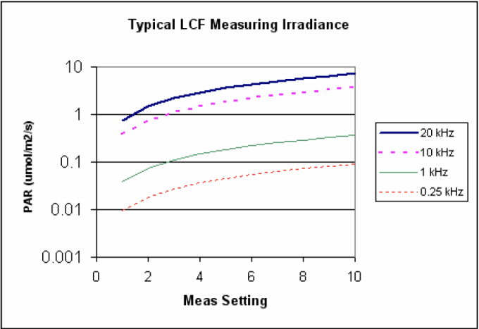
The measuring beam intensity is typically very small (0.02 and 0.2 μmol m-2 s-1 - see Figure 27‑59) because of the modulation. If the modulation is turned off, and the measuring beam setting turned up to 10, typical output is about 90 μmol m-2 s-1. However, the internal light sensor will usually not measure this accurately, since it is not calibrated for those two LEDs.
LCF Calibration Menu Programs
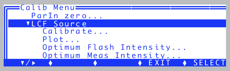
Fluorometer calibration routines are found in “Calib Menu|LCF Source”, but only when the <open> <light> <source> node specifies the 6400-40 LCF.
Calibrate...
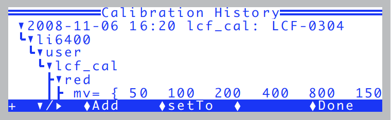
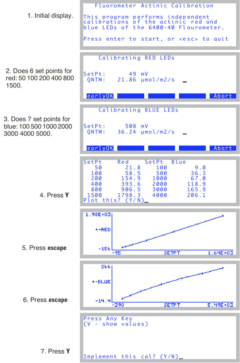
This calibration routine (Figure 27‑62) will generate the relation between red and blue control voltages and resulting quantum fluxes in the chamber. These relationships are used to compute first guesses for actinic control, as well as for subsequent computations of %Blue (viewed on display line g). Once started, the routine runs through a range of control settings for the red and blue LEDs separately. If you implement the results (step 7; Figure 27‑49), the calibration history will be updated (Figure 27‑61).
Plot
This routine plots the currently active relation between red and blue control signals and resulting in-chamber quantum flux. That is, it does steps 5 and 6 in Figure 27‑62.
Optimum Flash Intensity
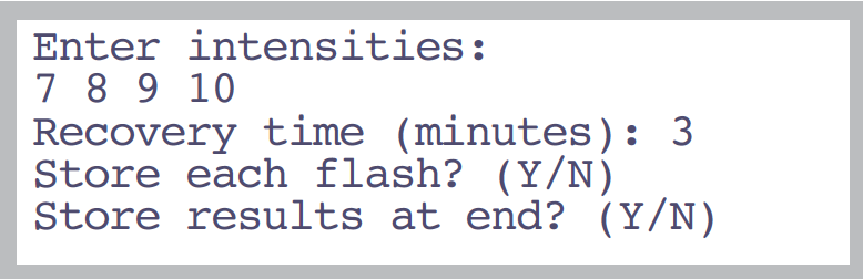
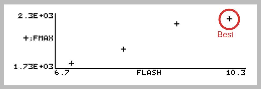
This program is designed to be an aid in determining the best flash intensity to use (Figure 27‑63). You are prompted to enter a range of flash intensities, and a recovery time after each flash. Run this program while clamped onto a representative, light-adapted leaf, and the program will, at the end, present you with a graph of Fmax plotted against flash intensity. Ideally, the optimum flash intensity is the lowest intensity value that yields the largest fluorescence value. If the highest intensity (10) causes the highest fluorescence yield, then your leaf is a good candidate for the MultiPhase Flash protocol (Using the MultiPhase Flash Protocol).
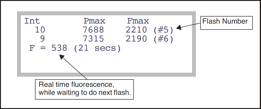
Once the program is running, the display will look something like .
After doing the list of flash intensities you asked for, you are prompted “Plot This (Y/N)”. A Y response will provide a plot of Fmax as a function of flash intensity, as shown in Figure 27‑65.
Optimum Meas Intensity
This program is designed to help you find the proper measurement intensity for determining Fo. That is, the intensity that is as large as possible without inducing photosynthesis.
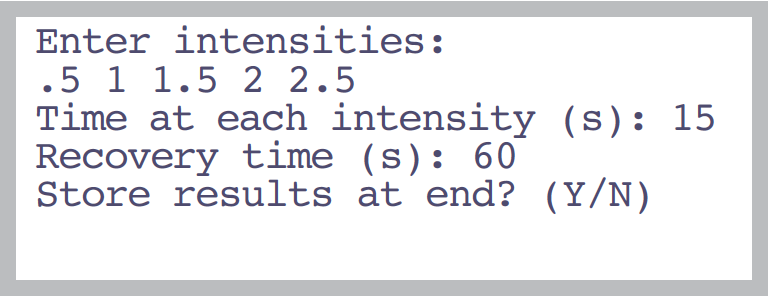
You are prompted for a series of measuring beam intensities (Figure 27‑66) to try. The time at each intensity is entered, as well as the recovery (measuring beam off) time. During the “time at each intensity”, the program collects fluorescence data F, then determines dF/dt (labelled “slope”). At the end, you are provided with a plot of these slopes as a function of measuring beam intensity.
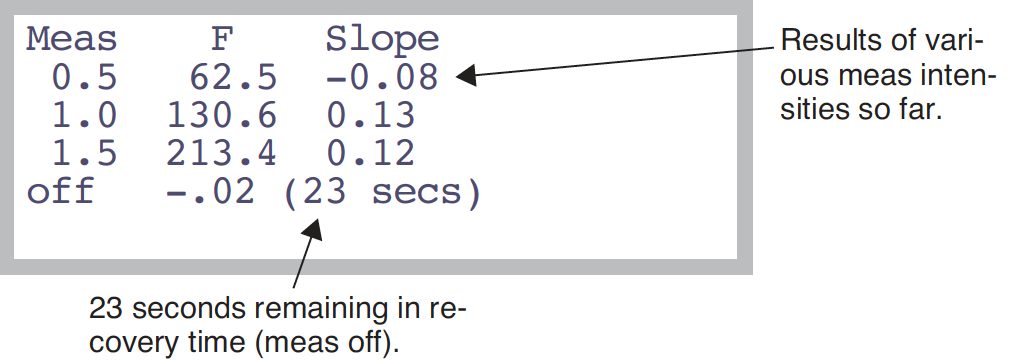
Once the program is running, the display shows measuring beam intensity (Meas), mean F, and dF/dt (Slope) (Figure 27‑67). During the recovery period, Meas will show “off”, and the time remaining.
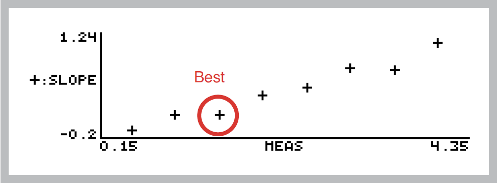
At the end, dF/dt as a function of measuring intensity is plotted for you (Figure 27‑68).
Square Flash Calibration
This automated routine is an important part of using the MPF method. In order to appropriately set the MPF parameters, an example rectangular square flash (RF) must be performed first (see Making Measurements). Getting nice square flashes out of the LCF requires calibration. To do that, clamp onto an example leaf (or use an empty or open chamber) and run the Square Flash Calibration in the LCF Calibration Menu (Figure 27‑69).
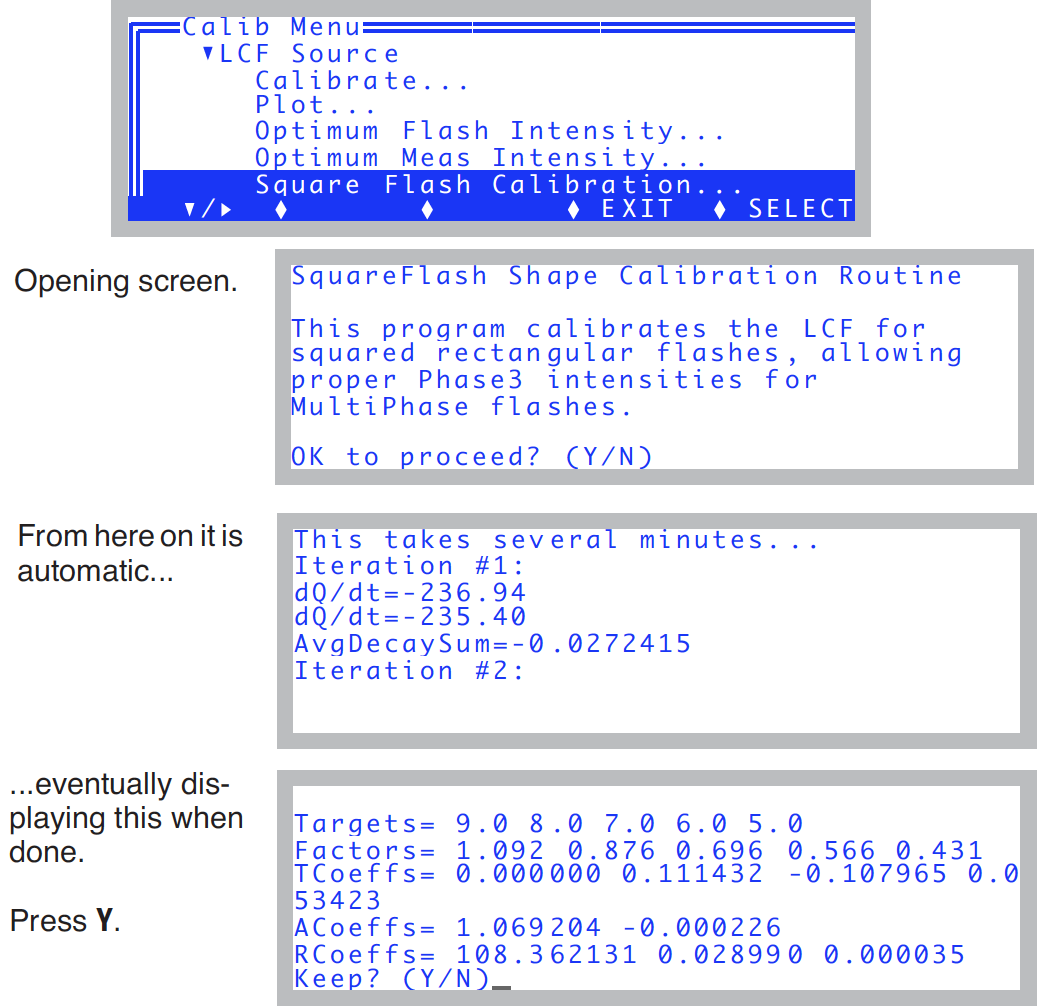
The reason1 this calibration is necessary is that LED efficiency drops with heating. When the LEDs in the LCF are turned on very brightly for a flash event, their output begins to fall almost immediately upon reaching their target brightness. We compensate for this by attempting to increase the current with time to the LEDs just enough to balance this. Unfortunately, the required “shape” of the control signal is not determined in real time, but must be predicted beforehand. Thus, the Square Flash Calibration routine runs the LCF through a variety of flashes of varying duration and intensity, and determines some empirical relationships that it can use later to provide reasonably square rectangular flashes, and reasonably square phase 1 and phase 3 portions of multi-phase flashes.
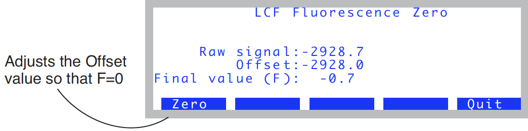
Zero Fluorescence Signal
This routine is used to zero the LCF fluorescence signal. The chamber does NOT have to be empty to do this.
View Factory Cal
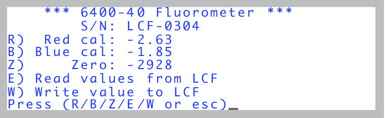
Each LCF has a unique calibration that relates the in-chamber light sensor’s signal to quantum flux. In fact, there are two calibration factors: one for the red LEDs, and another for the blue LEDs. They are measured at the factory, and reside in the memory of the LCF. This allows LCFs and consoles to be interchanged freely, without having to keep track of calibrations. The calibration stays with the LCF.
The “_View Factory Calibration” program allows you to view these values and even change them, although such changes are not normally recommended for the user.