Basic Experiments
The following experiments will guide you through a range of LCF operations. The first three experiments deal strictly with fluorescence, while the last two combine fluorescence with gas exchange. Before performing the first three experiments, verify the basic functionality of the LCF as described in Basic Functionality Test.
Fluorescence Experiments
These experiments cover some basic fluorescence measurements, such as determining quantum efficiencies for dark adapted and light adapted leaves, and serve as a good introduction to fluorometry with the LCF.
Experiment #1 Determination of Fv / Fm
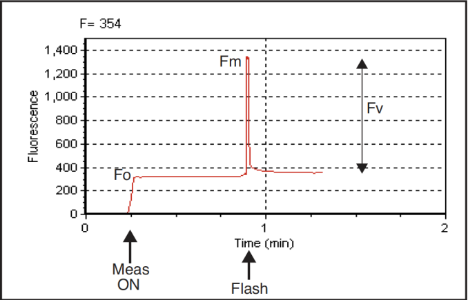
Fv/Fm is an estimate of the maximum quantum efficiency of PSII reaction centers. This ratio is calculated from two parameters: Fo and Fm. Fo is the fluorescence level of a dark-adapted plant with all PSII primary acceptors ‘open’ (QA fully oxidized). Fm is the maximal fluorescence level achieved upon application of a saturating flash of light, such that all primary acceptors ‘close’ (QA fully reduced). Variable fluorescence, Fv, is the difference between Fo and Fm. The variable to maximal fluorescence ratio is normally between 0.75 and 0.85, depending on leaf health, age and preconditioning.
- Dark-adapt the leaves
- The best technique for thoroughly dark adapting leaves is to leave them in complete darkness overnight. For illustration purposes, however, it may be adequate to use plants dark-adapted for at least 20 minutes prior to measurements of Fv / Fm.
- You may also wish to use the 9964-091 dark adapting clips.
- Set the appropriate LCF settings
- Check to make sure the LCF settings are appropriately set (f2 or f4, level 8), as in Table 27‑9.
- Logging?
- If you wish, open and name a log file (f1 level 1).
- Clamp the first leaf in the dark LCF
- The measuring light should be on (f1 level 9) and the actinic and far red off (f4 and f5 level 9). Monitor the fluorescence signal F on display line m. It should stabilize within a few seconds. Watch dF/dt on that same display line to indicate stability. Typically, when the absolute value of dF/dt < 5, F can be considered to be stable.
- If F doesn’t stabilize, the measuring intensity may need to be lowered. It is important that the modulation rate be low (0.25 kHz). The intensity of the measuring light needs to be set high enough for a measurable fluorescence signal, but not so high as to excite PSII and drive photosynthesis.
- Do FoFm
- After F has stabilized, press Do FoFm (f3, level 0). The status LEDs on the 37-pin connector will flash before and after the saturation flash, and a beep will sound when the data is logged (if you’ve opened a log file). Note the values of Fo, Fm, and Fv/Fm on display line n. Is Fv/Fm reasonable (0.75 to 0.85)? If it is not, it may be due to inadequate dark adaptation, or inappropriate fluorescence measurement settings.
- View the flash details
- Press View fsh/drk (f5 level 0) followed by view_Graph (f1) to view the flash. The detailed data collected at 20 Hz during the flash will be plotted versus time. Looking at the details of the flash makes it easier to determine if the settings were appropriate, and if the leaf material was adequately dark-adapted. Examples of “good” and “suspect” flashes are shown in Figure 27‑45. Note that there is an automated way of determining the appropriate flash setting. See Optimum Flash Intensity.
-
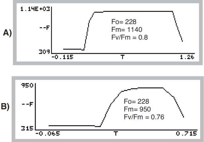
Figure 27‑45. A dark-adapted philodendron measured with two different flash settings. A) Example of a good saturation flash: flash length and intensity are appropriate for this leaf material. B) Example of a poor saturation flash: flash length was too short and intensity too small. Fv/Fm was underestimated by 5%. - Repeat with additional samples
- Repeat these measurements and try to compare results of different plants and healthy versus stressed plants (e.g. water or temperature-stressed).
Experiment #2 Determination of PSII efficiency
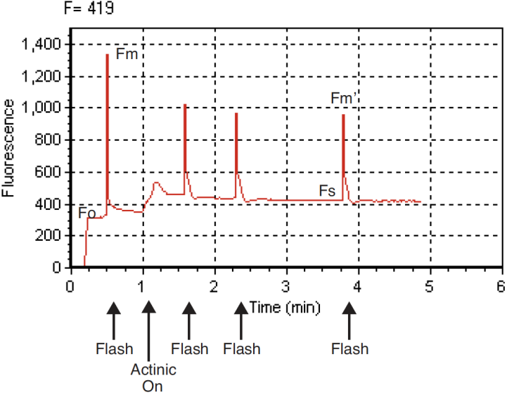
PhiPS2 (also called ΔF/Fm’) is the fraction of absorbed PSII photons that are used in photochemistry, and is measured with a light adapted leaf (Equation 27‑9). It is calculated from Fs and Fm’, where Fs is steady state fluorescence and Fm’ is the maximum fluorescence from a light-adapted sample upon application of a saturation flash (Figure 27‑46). See also Genty et al. (1989).
- Select light-adapted leaves
- For this exercise, select a light-adapted plant, that has had at least 20 minutes of acclimation at the desired light level. For the first part of this experiment, you’ll need several leaves that are about the same age and have similar illumination. At the end, you may want to try some leaves that have been at other light levels (e.g. shade vs. sun leaves).
- Set the proper LCF settings
- Use Flr Editor (f2 level 8) or Flr Adjust (f4 level 8) to set the measuring and flash settings (Table 27‑10). Also, adjust the actinic intensity to the leaves’ ambient level and turn it on (f5 level 2).
- Open a log file
- This is optional.
- Clamp onto the first leaf and equilibrate
- Wait until F (display line m) comes to steady-state. Watch dF/dt as in the first exercise. If you are using an actinic light intensity that is different than what the leaf was adapted to, you may need to wait 20 minutes or more until the leaf is acclimated to the new light level.
- DoFsFm’
- Once at steady-state, trigger a saturating flash to reduce any oxidized primary acceptors by pressing Do Fs Fm’ (f3 level 0). Fs and Fm’ can be viewed on display line o, and PhiPS2 on display line p. How does PhiPS2 compare with the Fv/Fm measured in experiment #1? (It should be lower, as is explained below.)
- View the flash details
- View the flash via (f5 level 0). The light-adapted flash should look similar to curve A in Figure 27‑45, but have smaller amplitude. More signal noise may also be evident. If the flash plot looks more like curve B, then the Flr Editor settings should be re-evaluated for your plant material.
- Repeat with other leaves
- Repeat steps 3 to 5, measuring leaves of similar age and light history.
- For further study: try different light values
- Compare PSII quantum yields of leaves adapted to high (2,000 μmol m-2 s-1) and low (100 μmol m-2 s-1) light levels.
Experiment #3 Determine Fv / Fm and Quenching Coefficients
Three other useful fluorescence parameters will be explored in this experiment. Fv’ / Fm’ (Equation 27‑10) represents the efficiency of energy harvesting by oxidized (open) PSII reaction centers in the light. Two competing processes that quench (decrease) the level of chlorophyll fluorescence in the light are referred to as photochemical (qP) and non-photochemical (qN) quenching (Equations 27‑13 and 27‑14). Many disciplines use these parameters, but the latter two are particularly useful as quantifiers in stress physiology research.
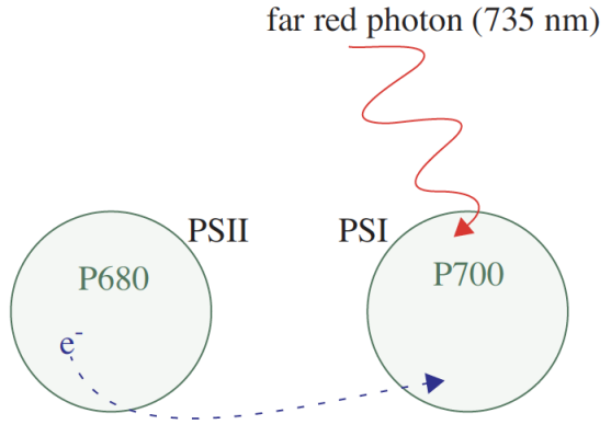
All three of these parameters require Fo’, the minimal fluorescence (in the dark) of a light-adapted leaf. How can this be determined? One method would be to allow the sample to dark-adapt and wait until all PSII centers oxidize (usually 20 minutes or more). A more expedient method (Figure 27‑47) would be to use far-red light to preferentially excite PSI and force electrons to drain from PSII. Only a few seconds of far-red time are needed for this to occur. The LCF provides a “dark pulse” routine which uses this second method to determine Fo’. See Figure 27‑22 for an illustration of the dark pulse timing parameters.
- Select some plants
- We’ll need both dark and light-adapted leaves for this exercise.
- Set LCF settings as in Experiment #1
- In addition to the dark-adapted settings used before (Table 27‑9), this exercise also requires configuring the dark pulse parameters (Table 27‑11) to measure Fo’.
- Clamp onto the first leaf
- With the actinic off and measuring light on, wait until F (display line m) becomes stable. (e.g., wait until | dF/dt | < 5.)
- Measure Fv / Fm
- Press Do FoFm (f3 level 0). Fo (display line n) is immediately set to the current value of F. Then a saturating flash is done, and Fm is set to the maximum value during the flash. Following the flash, the data is logged. Check the Fv/Fm value (display line n) and make sure it is reasonable. Finally, view the flash details (f5 level 0).
- Turn on the actinic light and equilibrate
- Set the actinic level to the average mid-day PAR value for your plant material. Let the plant adapt to the new light level for about an hour before going to the next step. To determine when the plant is adapted to the new light level, look for stability in F.
- Do FsFm’Fo’
- Press Do Fs Fm’ Fo’ (f4 level 0) to trigger the following sequence: set Fs, do a saturating flash and set Fm’, and then a dark pulse to set Fo’. When it is done (it will take about 12 seconds), view the flash details and check the new Fs, Fm’, and Fo’ parameters in group o. The light-adapted flashes should resemble plot A in Figure 27‑45.
- View the dark pulse details
- Assess whether the dark pulse settings were appropriate by checking to see if the fluorescence signal leveled off during the pulse (see Figure 27‑49).
-
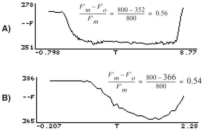
Figure 27‑49. A light-adapted bean leaf measured with two different dark pulse settings. A) Example of a good dark curve: far red intensity and time were appropriate for the leaf material (notice the curve flattened before the actinic light was turned on). B) Example of a poor dark pulse: far red intensity is not bright enough and time is too short to get a flat curve. This underestimates F’v/F’m by about 4%. - Compare Fv / Fm with Fv’ / Fm’
- Look at the calculated Fv’ / Fm’ value (display line o). Question: How should this value compare with the Fv / Fm values collected in Experiment #1? Answer: Fv’ / Fm’ should be < Fv / Fm, since Fv / Fm is the maximum light harvesting efficiency, and Fv’ / Fm’ is the actual light harvesting efficiency at some light level, which is reduced by competing processes for light energy.
- Examine the quenching coefficients
- The quenching coefficients, qP and qN, are located in display group p, and are described in Equations 27‑13 and 27‑14. qP and qN range in value between 0 and 1. For a truly dark adapted plant, qP = 1 and qN = 0 at the time Fv/Fm is determined. As light increases, these coefficients tend to move in opposite directions (see, for example, Figure 27‑52).
- Repeat steps 3-7 on additional leaf samples
- Compare the results with leaves adapted to high and low light conditions like the previous exercise. Question: Would you expect low or high light-adapted leaves to have more efficient PSII light-harvesting reaction centers? Answer: Normally, low light-adapted leaves will be more efficient at using the incident light. At low light intensities there is less excess PAR, allowing most plants to be more efficient at light harvesting.
Fluorescence and Gas Exchange Experiments
The next two experiments combine gas exchange and fluorescence. Make sure the IRGAs are zeroed and matched, and the instrument is ready to measure gas exchange. If you are not familiar with gas exchange measurements with the LI-6400, refer to Preparation Check Lists. This experiment uses AutoPrograms. If you are not familiar with these, the basics are discussed in AutoPrograms on page 9-29 in the instruction manual.
Experiment #4 Kinetic Experiment
The goal of this experiment is to take a fully dark-adapted plant and measure the progress of gas exchange, electron transport, and fluorescence quenching, while illuminating a leaf with high light.
- Dark-adapt plants
- It is best to use plants that have been dark-adapted overnight. At the very least, dark-adapt them for 20 minutes.
- Set up real time graphics
- We’ll want to plot the quenching coefficients against flash count. That is, QP (ID 4216) vs. FCnt (ID -84), and QN (ID 4220) vs. FCnt. Configure the real time graphics by pressing GRAPH Setup (f4 level 4).
- Set up an unused graphics screen with two XY Plots (QP vs. FCnt, and QN vs. FCnt). Use the default autoscale option. For details doing this, see Real Time Graphics on page 6-14 in the instruction manual.
- Prepare chamber environment
- CO2 - If there is a mixer installed, control at ambient (e.g. 370 μmol mol-1) values in the sample cell.
- Light - Set for a normal mid-day value (f3 level 8), but leave Actinic turned off (f1 level 9).
- Flow - Fixed at 300 μmol s-1.
- Prepare LCF settings
- Set for dark-adapted material, as determined in experiments 1 and 2.
- Clamp onto the first leaf
- Turn the measuring beam on and monitor F until it stabilizes. If F climbs steadily, the measuring beam intensity is probably too high.
- Run the autoprogram “AutoLog2”
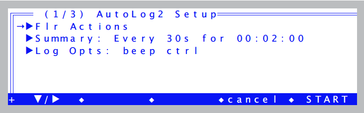
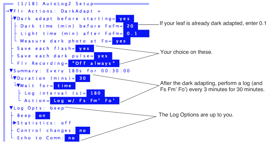
- Autoprograms are launched by pressing Auto Prog (f1 level 5). Select the one named “AutoLog2”. Once you’ve named the data file, you will be shown a setup dialog (Figure 27‑50).
- Set the values according for Figure 27‑51.
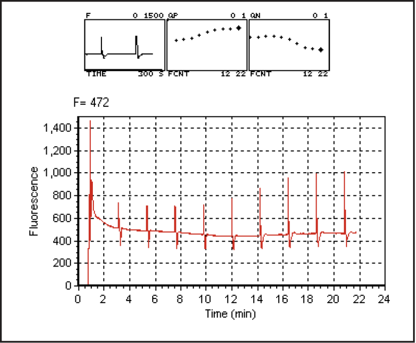
- Watch
- After starting the program(f5 Start), watch the real time graphics display (f3 level 4, or else ] ). Given enough time, a steady-state fluorescence level, Fs, and steady state photosynthesis rate should develop. What happens to qP and qN over time, after the actinic light turns on?
How long does it take for gas exchange to come to steady-state? (Compare this time to the time for the fluorescence parameters come to steady-state.)
Experiment #5 Light Response Curve
There can be many possible objectives in doing light response curves (see Light Response Curves). In this experiment, we will focus on two parameters, PhiPS2 and PhiCO2 (ΦPSII and ΦCO2 in Equations 27‑9 and 27‑11).
ΦPSII is the quantum yield of PSII calculated from fluorescence, while ΦCO2 is the quantum yield calculated from CO2 assimilation. In order to calculate this, we need to know total assimilation, which comes from measured (net) CO2 assimilation (Photo) in the light, and an assumption - or prior measurement - of assimilation in the dark (Adark). We also need absorbed PAR, which involves knowing incident PAR and leaf absorptivity (see Leaf Absorptance).
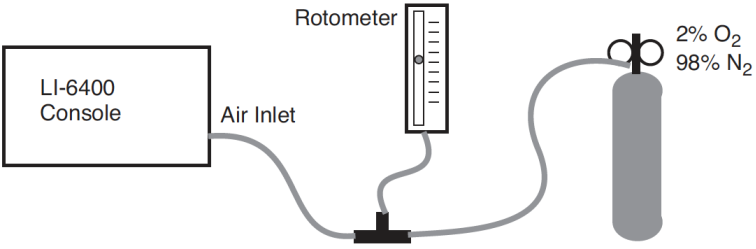
Note: If using a C3 species for this experiment, it is best to proceed under nonphotorespiratory conditions. That is, low oxygen. (For the plant, not you). This can be achieved by connecting a tank of 2% or less oxygen to the LI-6400 inlet, using an appropriate regulator, “T” fitting, and flow meter, to provide adequate flow for the pump, and a place for the excess flow from the tank to be vented (Figure 27‑53). If you do not do this, the measured relationship between and will likely not be linear. Don’t forget to change the OxyPct value in the LI-6400. Using a C4 plant avoids all of this.
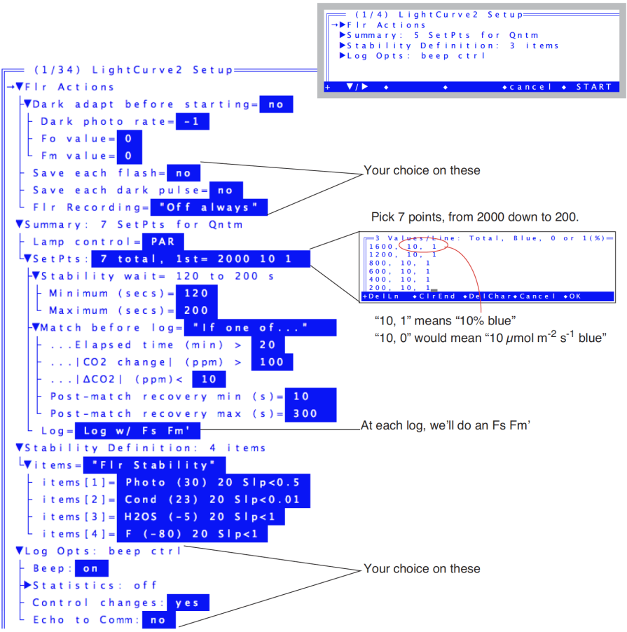
In this exercise we will start with a light-adapted plant and gradually work toward higher quantum efficiencies and yields by decreasing the incident light. We will use the AutoProgram “Flr Light Curve” to accomplish this.
- Set the environmental controls and LCF.
- Pick a light adapted leaf, and set the environmental controls as follows:
- CO2: (f3 level 2). Start with controlling on reference CO2 at 20 μmol mol-1 above ambient.
- Humidity/Flow: (f2 level 2) Start with fixed flow at 500 μmol s-1 and bypass most of the desiccant.
- Light: 2000 μmol mol-1, with 10% blue.
- Temperature: Block temperature set to ambient.
- LCF: Use settings determined in the previous exercises.
- Set the fluorescence constants
- Press Prompt All (f5 level 3 in New Measurements mode). Here are some suggested values:
- BlueAbs: Leaf absorptance in the blue. Use 0.92 (see Leaf Absorptance).
- RedAbs: Leaf absorptance in the red. Use 0.87.
- Adark: Photosynthesis rate in the dark. Use -1 μmol m-2 s-1.
- PS2/1: Fraction of photons that go to PSII. Use 0.5.
- Set up real time graphics to wait for stability.
- Wait for stable, flat lines in the conductance, photosynthesis, and fluorescence graphs. Also, display lines e and m, (or [ then C for the diagnostic mode stability display) can be checked for gas exchange and fluorescence stability parameters.
- Change to automatic control.
- Once the leaf has stabilized, check the value of H2OS (line a) and change the flow control (f2 level 2) to constant water mole fraction using the current H2OS value as the target. Also, change the CO2 control (f3 level 2) to target the sample cell, using the current sample cell value (CO2S line a) as the target.
- View the real time graphics for the fluorescence light curve.
- Press ] and view the real time fluorescence at f, and the PhiPS2-PhiCO2 plot at g.
- Launch the AutoProgram.
- Choose the program “Flr Light Curve” from the AutoProgram menu (f1 level 5). Name the file, then answer the prompts as indicated in Figure 27‑54.
- If you wish to save this setup before starting, press the labels key to get the second level of fct keys, and press saveAs. You could name the parameters Experiment#5, for example. If you wanted to run this again at a later date, you would load these parameters from LightCurve2’s setup screen by pressing Open... and picking the Experiment#5 file.
- Watch the light curve develop
- Press Start to launch the program, and watch the light curve develop. The real time graphics should be something like that shown in Figure 27‑55.
-
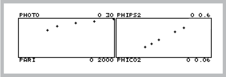
Figure 27‑55. Typical light curve real time graphics. The program does light from high to low, so the light curve (left) will develop from right to left, while the PhiPS2-PhiCO2 plot (right) will develop from left to right. - Graph data and calculate values
- After the last light level, press View File, (f2 level 1) to access GraphIt for your open data file. Press Import Config (f1) and choose “Light Curve”. The light curve (Photo vs. ParIn_μm ) will be drawn from the data (Figure 27‑56).
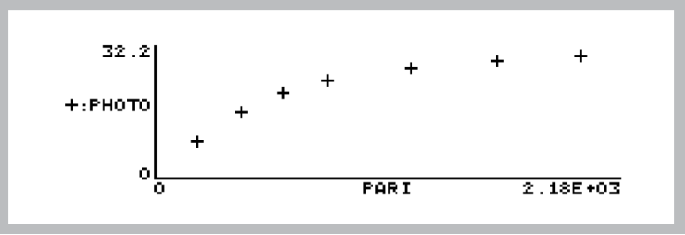
Now, plot PhiPS2 against PhiCO2. The quickest way to do this is to press Import Config (f1) and pick “PhiPS2 vs PhiCO2”. This will plot the points, and fit a straight line through them (Figure 27‑57). The relationship should be linear, with an intercept near zero and a slope > 8. For more information on this ratio refer to Chlorophyll Fluorescence References on page 27-90 in the instruction manual.
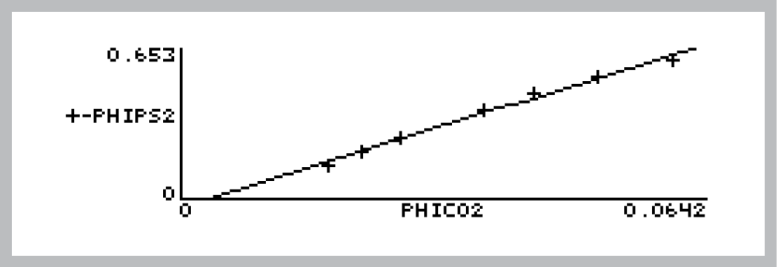
To view the slope and intercept, press View Data (f3), then C for Curvefit coefficients. For the data shown in Figure 27‑57, the intercept (Y axis) is -0.0234, and the slope is 11.0. (For details on finding slopes and doing curve fits with GraphIt, see Curve Fitting on page 12-14 in the instruction manual). When you press escape, you’ll be asked if you want to add the curve fit information to your data file.