Tour #5: Logging Data
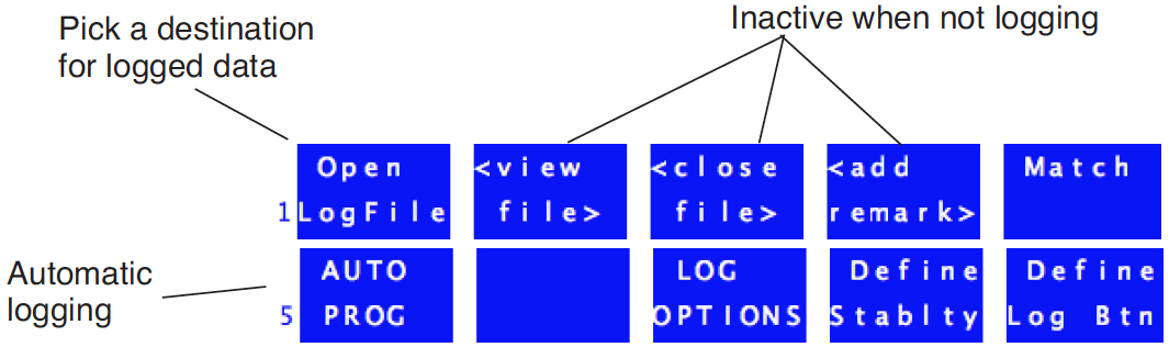
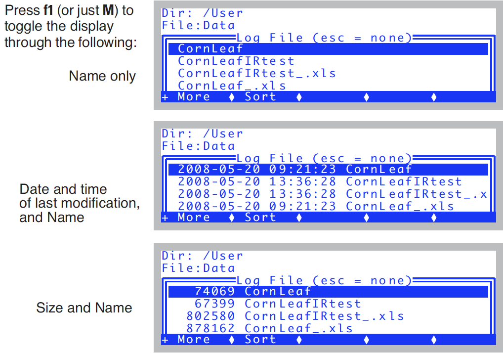
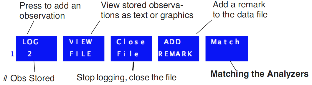
Recording data in New Measurements mode is discussed in detail in Chapter 9, but here we show the basics. Logging control functions are found on function key levels 1 and 5 (Figure 3‑53).
Logging Data Manually
Below is a step-by-step example in which we’ll open a file, and store some data.
Experiment #1 Log a data set manually
Start out in New Measurements mode.
- Press 1 (if necessary) to bring up the logging control keys
- Shown in Figure 3‑53.
- Press f1 (Open LogFile).
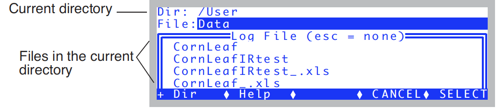
- This is how to select where data are to be recorded. Normally this is a file, but the comm port is also a possible destination.
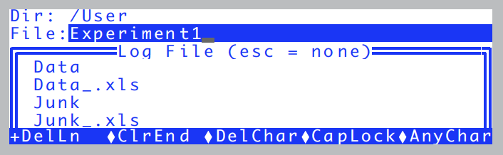
- The Standard File Dialog
- You are shown the Standard File Dialog. This screen will appear anytime you need to enter a file name. This dialog is fully described on page 5-9 in the instruction manual, but we’ll cover some important features of it here.
- The top line of the dialog shows the directory in the file system where you will be writing your log file. Normally, this should be /User. Below that is a list of the files in that directory. If you wish to change directories, press f1 (Dir).
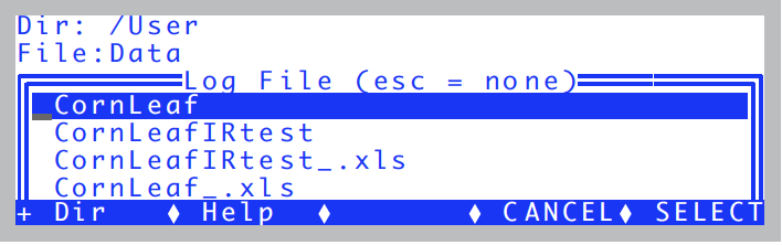
- Exploring the file list
- You can scroll through the file list, and even sort it, by pressing the up or down arrow key (▲ or ▼). The highlighted bar will jump from the file entry line to the list below, and you can then scroll up and down through the list, using ▲, ▼, home, end, pgup, and pgdn.
- While you are down in the file list, there are some things that you can do: Press labels, and you’ll see the second level of fct keys:
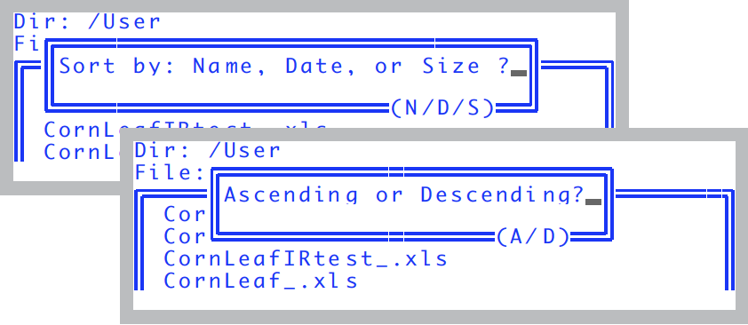
- Another thing you can do is sort the list. Press f2 (or just S). You can sort by Name, Date, or Size, and in Ascending or Descending order.
- Note that after the sort, the highlighted file remains the highlighted file; you’ll have to scroll up or down to see where you are in the list.
- Example: To find the most recently created or modified file in the list, press the following key sequence: S D D home. (That is, Sort on Date in Descending order, then jump to the top of the list).
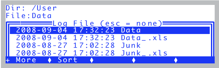
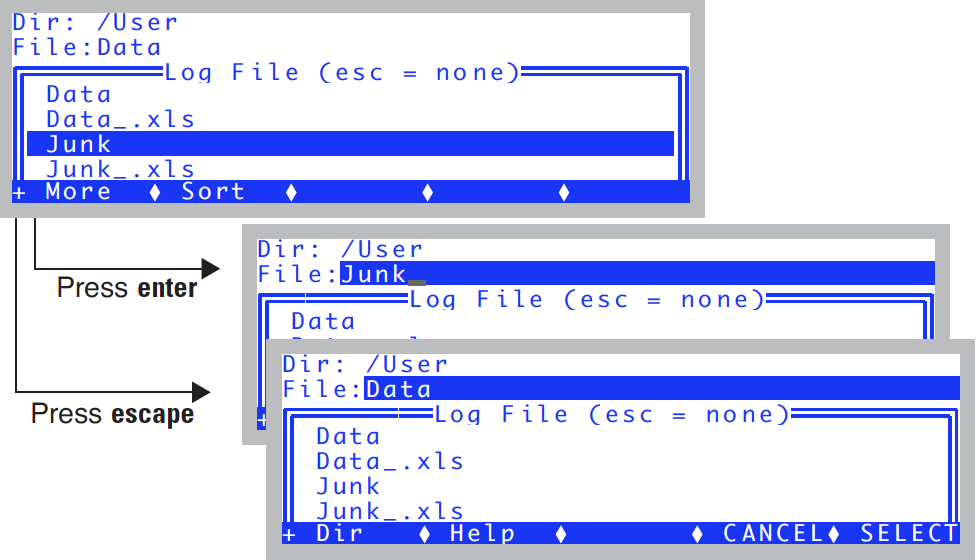
- You "exit" the bottom box by pressing enter or escape: If you wish to pick one of those existing files as the destination, highlight it, and press enter. Otherwise, just press escape and the file name entry line will remain unchanged (Figure 3‑57).
- Press labels to access the editing keys, then f1 (DelLn) to clear the default name, then type Experiment 1, and press enter.
- There are some illegal characters for file names (such as ’:’ and ’/’), but this dialog won’t let you type them. Spaces are ok.
- If you enter the name of a file that already exists, you will be given the choices of overwriting it, appending to it, or cancelling to enter a different name.
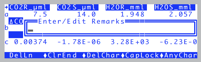
- Enter initial remarks.
- You’ll be shown the remark entering box (Figure 3‑59). Type a remark if you wish, and press enter.
- Redo Experiment #1 Humidity vs. Flow Rate.
- At each equilibrium value (that is, at the end of steps 4, 6, 8, and 9 of Experiment #1), press Log (f1 level 1) to record data at those moments.
- While the log file is open, the level 1 f1 function key label (Figure 3‑60) will show the number of observations logged.
- Graph the data
- Earlier we showed how to view strip charts of data in real time. Now we’ll show how to graph data you’ve recorded before closing the data file.
Viewing Stored Data
It is convenient - and sometimes necessary - to examine the specific data that has been logged, to see if the experiment is going as planned, or if an adjustment (such as a career change) is necessary.
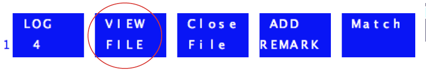
When logging is active (to a file), you can view logged data by pressing View File (f2 level 1).
Experiment #2 View Data Logged Thus Far
You can view data in your log file right from New Measurements mode, as long as the file is still open.
OPEN’s Graphics Packages
OPEN uses two graphics packages: Real Time Graphics is used to plot measurements as they happen. GraphIt, on the other hand, is only used with data that is stored in a file.
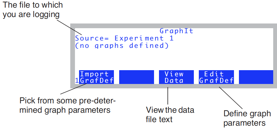
- Access GraphIt
- Press 1 (if necessary), then f2.
- After a few seconds, you will see something like Figure 3‑45.
- This is GraphIt, a useful program that appears in several contexts, and is explained thoroughly in Chapter 12 in the instruction manual. For now, just follow along, and we’ll make some graphs.
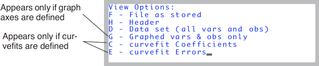
- View the data file as stored
- Press f3, then F (Figure 3‑62).
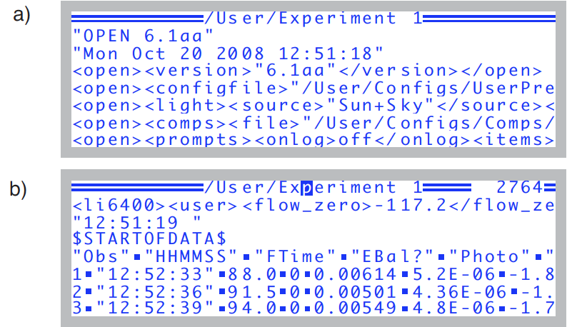
- After pressing F, you should see something like Figure 3‑63a. If you press pgdn, you’ll see more of the file (Figure 3‑63b).
- The little blocks (•) are tab characters, which is the default delimiter.
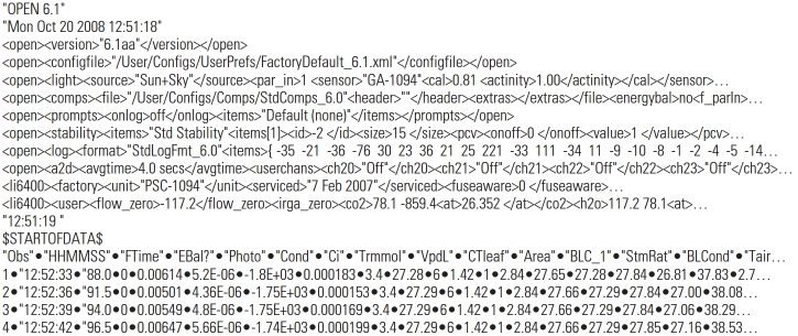
- If you could see all of the file at once, it would look like Figure 3‑64. If this seems an inconvenient way to view the data, keep reading (it gets better).
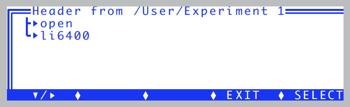
- View the Header
- Press escape to stop viewing the file “as stored”, and then press H (for Header). You will see, in convenient tree form, all the configuration and calibration information for the system as it was when you opened the file (Figure 3‑65).
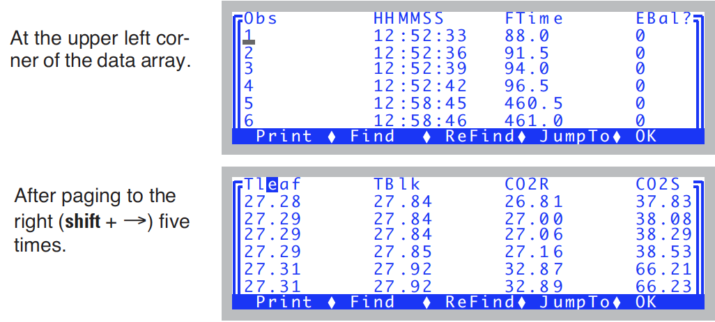
- View the data file in columns
- Press escape to stop viewing the header tree, then press D (for Data Set). You will see a more legible display (Figure 3‑66).
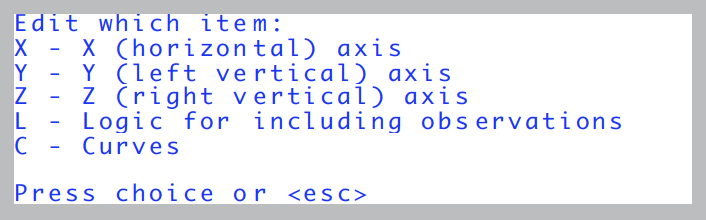
- Define a plot
- Press escape twice to stop viewing the data in columns and return to Graph-It’s main screen. Then press f4 (Edit Config) to define the axes for the plot.
- Put Flow on the X axis, autoscaled
- Press X. If you are presented with
V - change variableR - change range- then press V. (This choice will not appear if the X axis is currently undefined.) You will see a menu of variables, obtained from the label line in the data file. Scroll down (probably 5 pgdn’s from the top) until you find Flow. Highlight it and press enter.
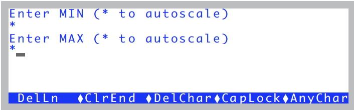
- Now set the range. (If you had to press V to change the variable, you’ll have to press R now to set the range.) You’ll be asked for the minimum and the maximum of the axis (Figure 3‑68). For each, just press enter to accept * for the value.
- When you are done, if the display does not return to the menu shown in Figure 3‑68, you’ll have to press escape.
- Put RH_S on the Y axis
- Press Y to pick a Y variable. (If you get the V/R choice again as in Step 6, press V). Highlight RH_S, and press enter.
- Now press escape to signal no more Y variables (you’ll be asked for up to 5 variables for this axis, and you only want one).
- Now enter * for the Min and again for the Max. (If the min and max are not automatically asked, press R to do this).
- Press escape until you get back to GraphIt’s main screen.
- Plot the graph
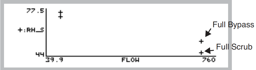
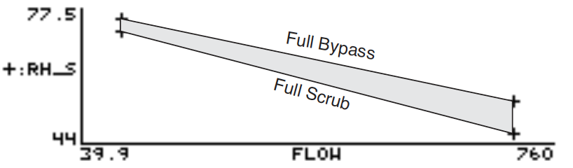
- If it didn’t plot automatically upon leaving the configuration editor, then press f2 to plot the graph (Figure 3‑69).
- These data illustrate the concept of an operating envelope for humidity control; if we draw a line around these data, we draw the envelope (Figure 3‑70).
- Save this definition for future use.
- Press escape to stop viewing the graph, and return to GraphIt’s main screen. Press f5 (Config SaveAs), and name the file “
RH & Flow”. (Storing this file uses the Standard File Dialog again, just as you saw when you opened a log file.) - Quick! Plot something else!
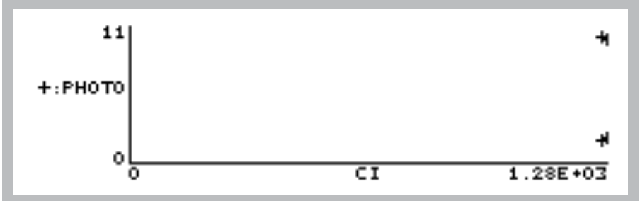
- From GraphIt’s main screen, press f1 (Import Config). You’ll be presented with a menu of plot definitions, which should include “RH & Flow”, or whatever you named it in the last step. Just for fun, let’s pick another one. Try selecting “A-Ci Curve” at the top of the list. You’ll get a very uninspiring plot (Figure 3‑71) but it illustrates how to quickly change plot definitions.
- Replot RH and Flow…
- Press escape, then f1 (Import Config), and select “
RH & Flow”, to redraw to our first plot. - …and view the plotted data
- Instead of pressing escape to stop viewing the graph, you can press V, and a scrollable menu of the data points that are plotted will appear (Figure 3‑72).
- Press escape to exit from this.
- Return to New Measurements mode, and close the file
- Press escape until you get back to New Measurements Mode, then press f3 (Close File).
That concludes the introduction to GraphIt, the tool for viewing logged data. It is accessible from New Measurements mode for a file that is open for logging, and also from the Utility Menu for previously logged files. GraphIt is fully described in Chapter 12 in the instruction manual.
Automatically Logging Data
OPEN’s mechanism for automatic operation is the AutoProgram. An Auto-Program is a list of instructions that the instrument should do, which typically includes setting controls and logging data. OPEN includes a small collection of AutoPrograms for various common tasks (described in AutoPrograms on page 9-29 in the instruction manual), but you can modify these and add to the collection.
Experiment #3 Log Data At Regular Intervals
We’ll demonstrate AutoPrograms with one that logs data at regular intervals. Start in New Measurements mode.
- Open a data file
- Press Open LogFile (f1 level 1) to name and open a data file.
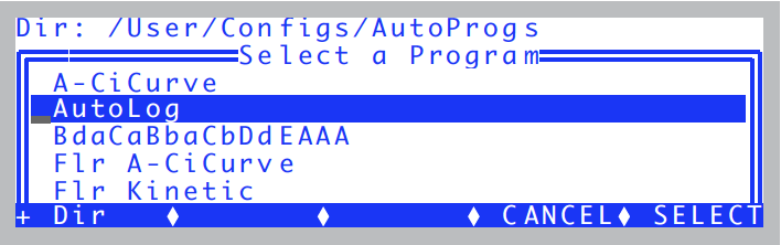
- Pick the AutoProgram “AutoLog2”
- Press 5 then f1. A menu of AutoPrograms will appear. Select the one named AutoLog2, and press enter (Figure 3‑73).
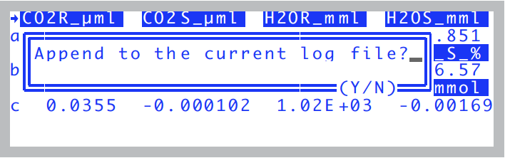
- Append to current log file?
- Whenever you launch an AutoProgram with a data file open, you’ll be asked if you’d like to append to that file (Figure 3‑74).
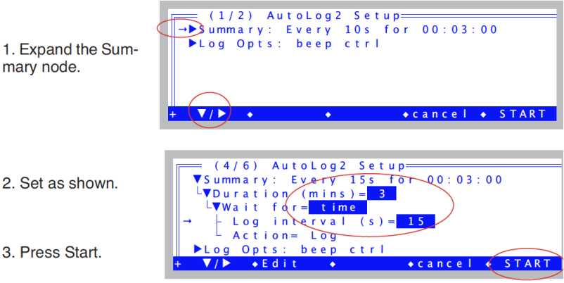
- Configure the program
- You will be shown a configuration screen (Figure 3‑75). Set it to log every 15 seconds over 3 minutes.
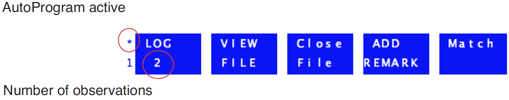
- Watch
- Press 1 to view the Log key label. Every 15 seconds, the number of observations will increment by 1.
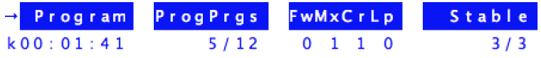
- Press K to watch the AutoProgram status line (Figure 3‑76).
- Normally, Program shows the number of seconds until the next event (typically, that event is data logging) will happen, and ProgPrgs (“Program Progress”) shows the number of logging events so far, and the total number when done. With AutoLog2, however, Program shows the time remaining in the whole program.
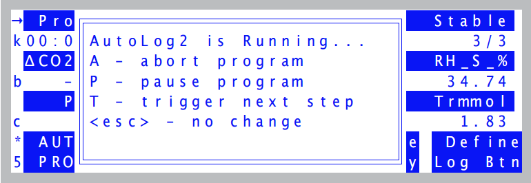
- Terminate it
- To stop an AutoProgram before it is done, press escape, then A (Figure 3‑77).
- Notice the T option in Figure 3‑77. Normally, this triggers the next step in an AutoProgram. With AutoLog2, however, it too will terminate the program. (If you want to log early with AutoLog2, just press the Log key.)
- Close the data file
- Press 1 then f3 (Close File) to do this. Notice that AutoPrograms don’t automatically close data files. You can open a file for logging, then run several AutoPrograms, accumulating data in that file. However, if you launch an AutoProgram without having a log file open, you will be asked to open one. A complete discussion of AutoPrograms is in Chapter 9 in the instruction manual.
Stability
An important question concerning data logging is when to do it. That is, do I log now, or should I wait longer for things to be more stable? Manual logging usually involves that question being handled at some conscious level by the operator. Running an autoprogram, however, leaves that decision to the machine.
Are there objective criteria that can be used by both the machine and the operator to decide on stability?
We wouldn’t ask that if the answer weren’t yes, and indeed, OPEN provides a fairly powerful technique for you to define and use stability criteria. f4 level 5 (Define Stablty) lets you select your standards for stability, and we’ll go there next.
Experiment #4 Set Up System Stability Criteria
Start in New Measurements mode.
- Press f4 level 5.
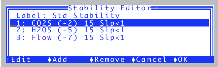
- You’ll see a screen similar to Figure 3‑78, listing the current stability criteria.
- Each variable to be considered is listed, along with the time period and relevant thresholds.
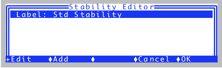
- Clean out the list
- If there are items in the list, highlight each and press Remove (f3) until there are none. This is not normal operating procedure, but it gives us a clean slate to work with.
- Build a definition
- Now, we need a definition of stability. An obvious one would be to look at photosynthesis and conductance. Over the course of a minute, if photosynthesis changes by less than 0.1 μmol m-2 s-1, and conductance changes by less than 0.05 mol m-2 s-1, then we could consider that stable.
- For purposes of an introductory tour, however, let’s pick reference cell CO2, sample cell CO2, and leaf temperature. (There’s no logic to this combination, but it’ll work fine for our example.) A good rate of change threshold for the CO2 values might be 1.0 ppm per minute, and 0.1 degree C per minute for the leaf temperature.
- We have been referencing rates of change as “per minute”. Does this mean we have to wait 1 minute after stability is achieved to see if it holds? No. Instead, we’ll specify some time period, such as 10 or 20 seconds, over which OPEN will keep running statistics; at any instant, if the rates of change over the last 10 or 20 seconds meet our criteria, then stability is reached.
- There is a danger to doing it this way, however. A fluctuating signal could happen to have a rate of change near zero for an instant during a transition from “going up” to “going down”, which could cause an AutoProgram to be fooled into logging too soon.
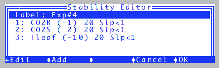
- We can prevent this by specifying a second parameter, such as standard deviation or coefficient of variation, in addition to a rate of change (hereafter called slope, or abbreviated Slp). Table 3‑3 illustrates our “tour stability criteria”, designed to avoid being fooled by a fluctuating signal.
-
Table 3‑3. Example stability criteria. Quantity Slope St Dev CO2R < 1.0 < 1.0 CO2S < 1.0 < 1.0 Tleaf < 0.1 < 0.1 - Add CO2R, CO2S, and Tleaf to the list
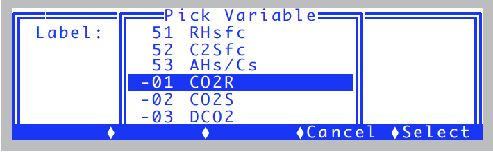
- Press the Add function key (f2). A list of variables will appear (Figure 3‑80).
- Select
-1:CO2R, and press enter. Press Add (f2)again, and this time select-2:CO2S. Do it a third time and select-10:Tleaf(Figure 3‑81). - Notice the default setting for each item is to check for slopes, with a threshold of 1.
- Change the label
- Set the label to Exp#4.
- Want to make changes?
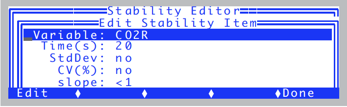
- Highlight CO2R, and press Edit (f1) or enter (Figure 3‑83). Here we see the options for each item in the stability list: the variable (quantity to be tracked), time period (seconds), coefficient of variation (in percent), rate of change (per minute), and standard deviation.
- This is how you can select the time period, and enable or disable any combination of the three possible statistics for a variable. Press Done (f5) to exit the Stability Item Editor.
- Exit the editor
- Press OK (f5) to exit the Stability Editor, and return to New Measurements mode.
- In the next part of the tour, we’ll see how to check on the system’s stability during operation.
Experiment #5 Monitor Stability In New Measurements Mode
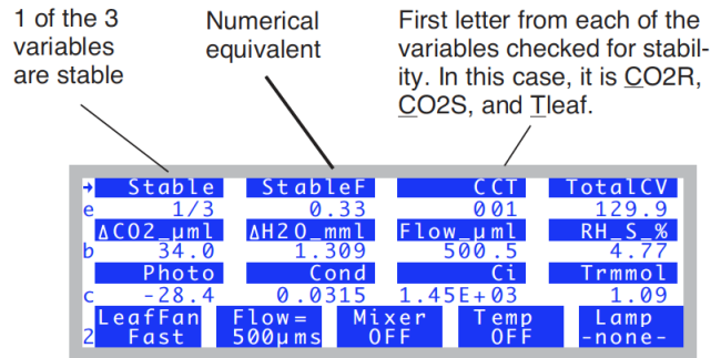
- Bring up display line ’e’
- Display line e contains two system variables that tell you moment by moment if the system has achieved your definition of stability. In the example in Figure 3‑84, one of the three is stable.
- Close the chamber, Pump On, Soda Lime Full Scrub
- Close the chamber, turn on the pump, put the soda lime on full scrub, and watch display line e, as one by one, the variables become stable.
- If you are thinking that waiting for “000” to become “111”, or “0/3” to become “3/3” is not particularly informative, we’d agree.
- There is a way to see the details of your stability checking:
- Diagnostic Mode, Screen A
- Press [ (left square bracket) to enter Diagnostics Mode. (That’s the short cut. The long way is to press 6, then f5, labelled Diag Mode). You should see something like Figure 3‑85. (If not, press A, and it will come into view.)
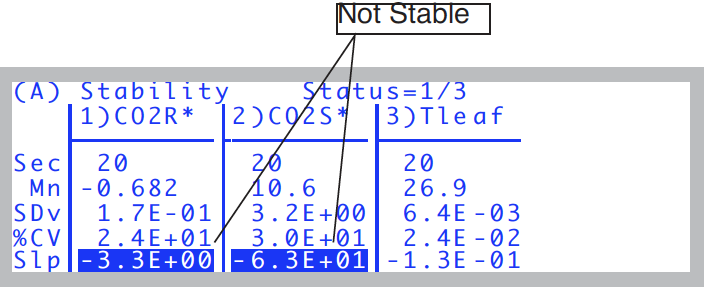
This is one of several diagnostic screens. (Quick Lesson: You press letters a, b, etc. to jump between the screens in diagnostics mode. To leave diagnostics mode and return to the normal New Measurements text display, press [.) In diagnostic display A, you can monitor all the details of your stability criteria.
When a variable is not stable, it is marked with an asterisk, and the reason (such the rate of change too large) is highlighted. Thus, there are two ways to check on stability: line e for a quick glance, or [ (then a, if necessary) for the details.
For more on Diagnostics Mode, see Diagnostics on page 6-24 in the instruction manual.
AutoPrograms, Stability, and Matching
Most of the default AutoPrograms can make use of this stability feature, and it takes the form of a Stability Definition node in the setup window. To see an example, try the next experiment.
Experiment #6 View stability and matching setup in an AutoProgram
- Re-open AutoLog2
- Re-open AutoLog2, but do not launch it yet.
- Change from time to stability
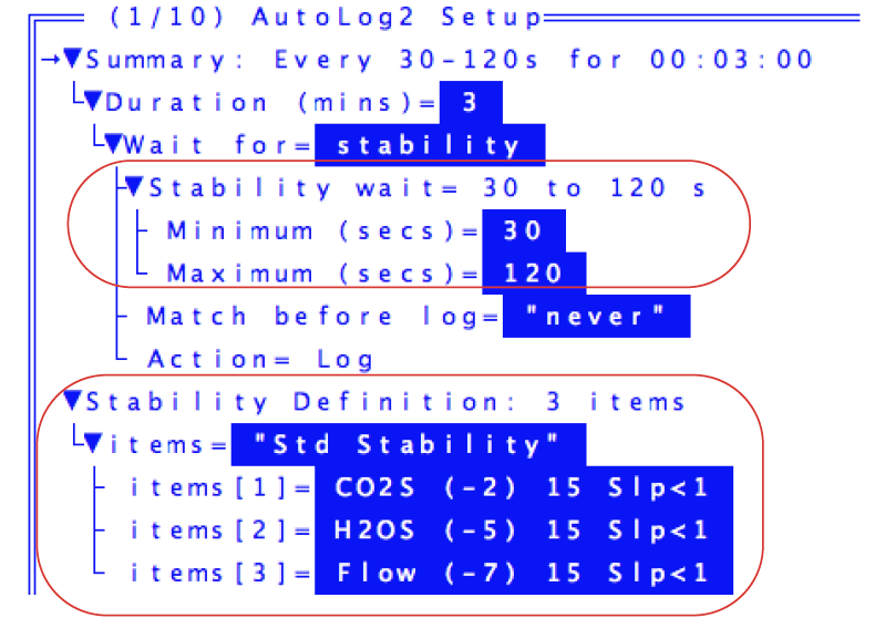
- Change the node Wait for from time to stability (Figure 3‑86). There will be some extra nodes that appear.
- Stability wait contains the minimum and maximum waiting times for stability to occur. Stability Definition contains the stability definition that will be implemented if the AutoProgram is launched. Note that this definition is not necessarily the currently active one - it is independent, and stored with the AutoProgram’s other parameters. If you launch the AutoProgram, its stability definition is implemented, and remains in effect once the AutoProgram finishes.
- It will be the stability definition present the next time that AutoProgram’s setup screen appears AutoPrograms use stability along with a minimum and maximum wait time.
- When logging (each point on a light curve, for example), the program will wait the minimum time (after setting a new light level), then start checking stability and log when the stability definition is met. If this doesn’t happen by the maximum time, it will log anyway, and move on to the next step.
- You can change the currently active stability definition anytime, even while an AutoProgram is running.
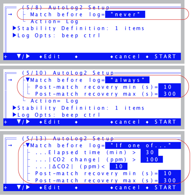
- Navigate up to the Match before log node
- This is the node that control matching. Navigate to it and press f2 (edit). You will see it toggles through three settings (Figure 3‑87).
- These are your matching options for AutoPrograms that have this node: you can never match, always match before logging, or only match if certain conditions are met. The conditional match occurs if at least one of the conditions is met: a) time since last match, b) change in CO2 since last match, or c) a small CO2 differential (the smaller the differential, the more important the match).
- When matching does occur, there is a post-match recovery time to allow stability to be re-achieved, and the minimum and maximum wait times for that are editable.
- Cancel the AutoProgram
- Press f4 (cancel).
Log Options
The next stop on the data logging tour will look at Log Options.
Experiment #7 Log Stability Variable Statistics
Start out in New Measurements mode.
- Access Log Options
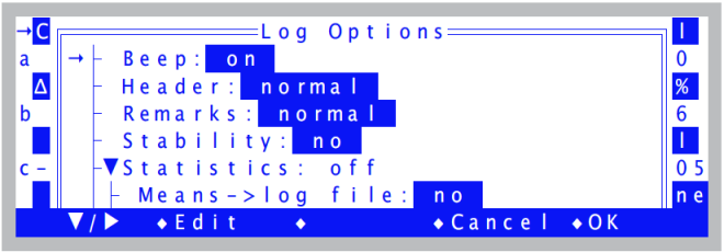
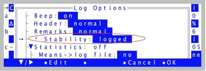
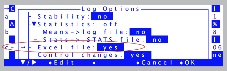
- If you have a log file open, close it (f3 level 1). Log Options is f3 level 5. When you press it, you will see something like Figure 3‑88.
- The entries in this menu give you several options for how your log file will look, and what is logged. The details are discussed in Log Options on page 9-14 in the instruction manual, but for now, focus on the fourth item, Stability Details. Setting this to Logged (Figure 3‑89) by highlighting it, and pressing Edit or enter, will cause the details (mean, standard deviation, coefficient of variation, and rate of change) of your stability variables to be included in your log file with each observation.
- Enable Stability Details
- Highlight
Stability, and press Edit (f2). The line should change toStability: Logged. - Exit Log Options
- Press OK (f5) to leave Log Options.
- Open a log file, and log a couple of dummy observations
- Press 1 then f1, and enter a destination file name, remarks, etc. Then press f1 (Log) a couple of times to log some data.
- View the file
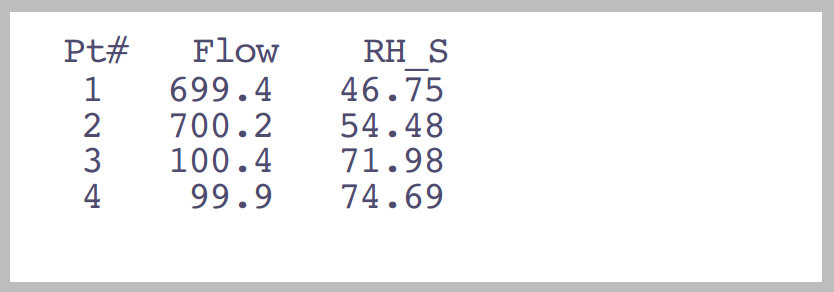
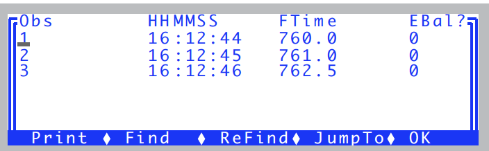
- Press f2 (View File), then f3 (View Data), then D (view Data set). You should see the first 4 columns of the data file:
- Now scroll to the right by pressing shift + ►. (You can get to the end of the line quickly by pressing shift + end). Eventually, you’ll see something like Figure 3‑91.
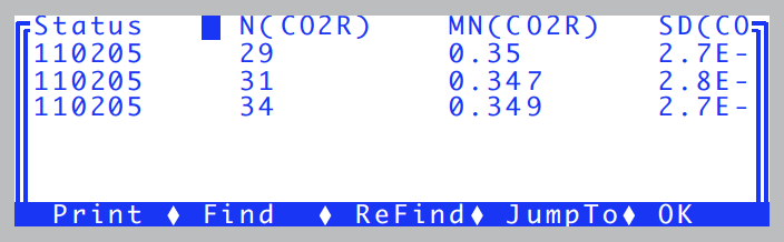
- Status is normally the last column. There will be 15 columns appended, containing the stability details. For each of the CO2R, CO2S, and Tleaf stability variables, there will be a N(), MN(), SD(), CV(), and SLP() columns, with the variable name in the parentheses (). N() is the number of samples, MN() is the mean value of those samples, SD() is standard deviation, CV() is coefficient of variation, and SLP() is slope, or rate of change.
- Return to New Measurements
- Press escape three times to get back to New Measurements, then close the file by pressing f3 (Close File).
- If you wish, you can go back and turn off stability logging now, or just leave it. The Log Options always revert back to their default settings at power on.
Experiment #8 Make an Excel File
You may have noticed one of the log options is Excel File: This option (which by default is Yes) creates an Excel version of your data file - with all equations built-in - in addition to the normal text version. For example, with this option set to Yes, when you open a log file named Data, there will also be another file created named Data.xls.
- Access Log Options
- If you have a log file open, close it (f3 level 1). Then access Log Options (f3 level 5) (Figure 3‑92).
- Create an Excel file (if necessary)
- If the Excel File option has been enabled, and you have logged some data, you will already have an Excel file to work with. Otherwise, set it to Yes, and go open a log file (f1 level 1), log some data, and close the file.
- Move an .xls file to your computer.
- If you haven’t done this before, there are many options, depending on your computer (Windows, Mac OSX, Linux), and whether you have a LI-6400XT or not (Ethernet or RS-232); this is all spelled out in detail in Chapter 11 in the instruction manual. For purposes of this step, we will assume you have made either a direct Ethernet connection between the LI-6400XT and your PC, or else both are plugged into the same local sub network.
-
- To verify you are connected, and to see your host name and IP address, access Network Status in the Utility Menu (Figure 3‑93).
- Connect the LI-6400XT file system to your computer using Windows Explorer (Figure 3‑94) or Max OS X Finder (Figure 3‑95).
- For Windows:
- For macOS:
- Navigate to the User directory
- Drag the Excel file you like to view to the desired folder on your PC, and open it with Excel (Figure 3‑96).
- You could simply double click it to open it without moving it to your PC, but, note the cautionary box on the next page.
- Change leaf area, and see it recompute automatically for that row.
- Note that some columns are marked "in", and some are marked "out" (row 10). The "outs" have equations associated with them so are computed, and the "ins" are simply inputs. Thus, if you change an input value, such as Area (column M), all the out columns in that row that are a function of area (such as Photo, column G) will change automatically.
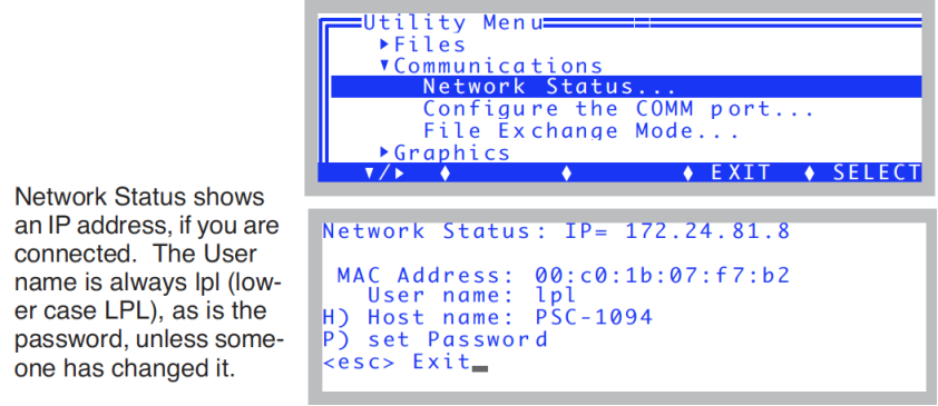
Figure 3‑93. Network Status. 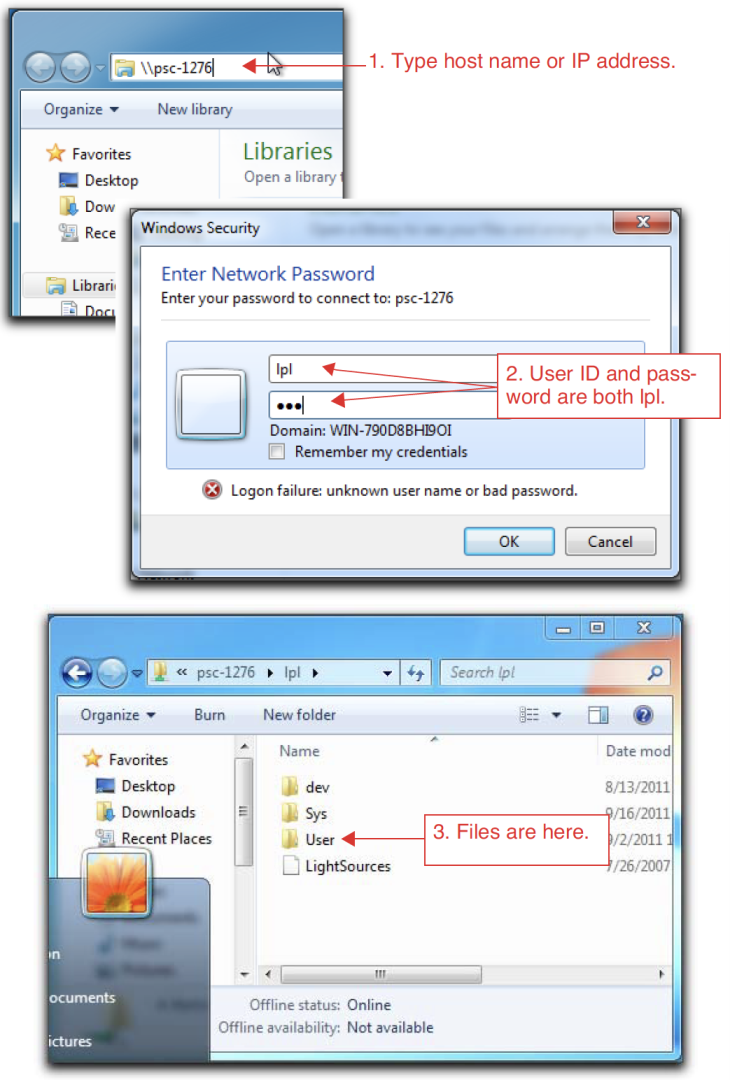
Figure 3‑94. Connecting to the LI-6400XT file system using Windows. 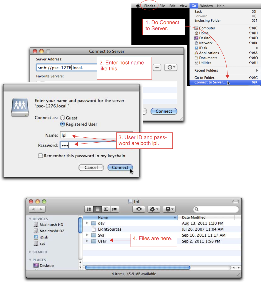
Figure 3‑95. Connecting to the LI-6400XT file system using Finder. 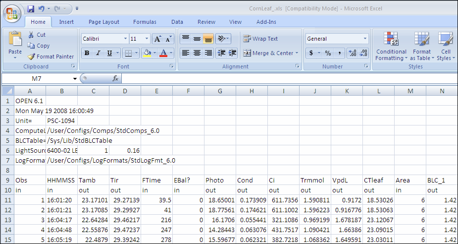
Figure 3‑96. Sample .xls data file. Columns marked with "out" (Row 10) are defined by equations.
Opening an Excel file that is on the console
This is OK.
This is OK even if the file is still active. However, as new observations are logged, you will not see them in Excel unless you re-open the file each time you want to check on it.
One thing to avoid if it is still an active file: Do NOT write to it. That is, do not overwrite the .xls file on the console. (Save it as an .xlsx, or save it somewhere else, but don’t write to the original while it is still being used by the LI-6400, or it may become corrupted.)