Tour #3: Controlling Chamber Conditions
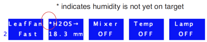
Chamber conditions are controlled from New Measurements mode via the function keys on level 2 (Figure 3‑24).
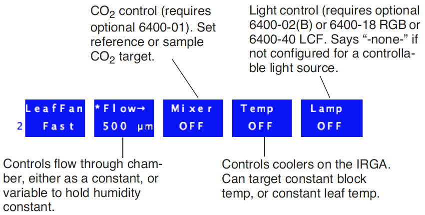
The main control areas are wind speed, flow/humidity, CO2, temperature, and light. The key labels for f2 through f5 indicate the current state of the control, along with the target value of active controls. This tour will acquaint you with each control. (Details of OPEN’s chamber control are given in Chapter 7 in the instruction manual.)
Fixed Flow Operation
Flow and humidity are grouped together into one control. You can specify a fixed flow rate (and let humidity vary) or a fixed humidity (and let flow vary).
Confused? Keep reading.
Experiment #1 Humidity vs. Flow Rate
This experiment illustrates the relationship between chamber humidity and flow rate.
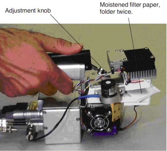
- Simulate a leaf with filter paper
- Use Whatman #1 filter paper (or even towel paper), folded a couple of times, and moist but not dripping. Clamp your “leaf” into the leaf chamber (Figure 3‑25). Use the adjusting nut to make the chamber seal snugly, but not too tight.
- Set soda lime to full bypass, desiccant to full scrub.
- The soda lime tube should be the one closest to you on the left side of the console. Roll the adjustment knob toward you for bypass. On the desiccant tube, roll the knob away from you for scrub. There’s no need for strong fingers here; when the knob gets resistive at the end of its travel, quit. It’s far enough.
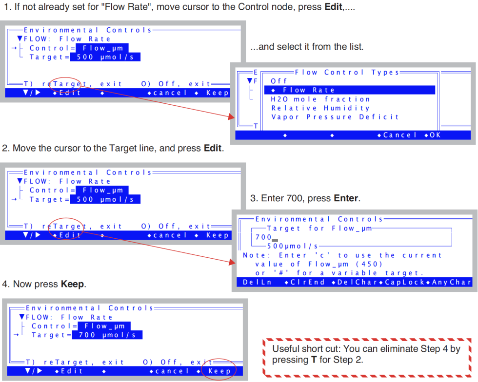
- Use a high flow rate: 700 μmol s-1
- Press 2 (if necessary, to bring up the level 2 function keys). Then press f2, select a flow rate of 700 (Figure 3‑26).
- Note the reference and sample water vapor channels
- If it’s not already there, put display line a on the top line. The two variables
- on the right (H2OR_mml and H2OS_mml) are reference and sample water mole fractions, in mmol mol-1. The reference should be near zero, since we are forcing all the air through the desiccant. The sample in this illustration is near 15 mmol mol-1; what your value is depends on how wet the “leaf” is, what the temperature is, etc.
- Note the flow rate and relative humidity
- Put display line b on the second line. Line b contains the flow rate
- (Flow_μml), which should match (usually within 1 μmol s-1) the target value shown on the flow control function key label (f2 level 2). Another item on line b we’ll be watching is relative humidity in the sample cell, in percent (RH_S_%).
- Change the desiccant to full bypass
- Observe what happens when you change the desiccant from full scrub to full bypass. The reference water vapor concentration (H2OR_mml) will increase to the ambient value, since we are now not drying the incoming airstream at all. The sample water vapor concentration (H2OS_mml) will not increase as much, since the paper is not able to evaporate as much water into the more humid air.
- Change to a low flow rate: 100 μmol s-1.
- Press f2 then type 100. (Notice the short cut: when you aren’t changing control modes, you can just start typing the target value after you press the function key. In our case, we didn’t need to press F again to specify fixed flow mode.)
- Note the sample and reference humidities
- The reference value hasn’t changed, but the sample value increased. Why? Because the air is going through the chamber at a much slower rate, providing a longer exposure to the evaporating paper. In fact, you may start getting “High Humidity Alert” flashing on the center line of the display. If it does, ignore it.
- Turn the desiccant to full scrub
- Observe the reference and sample humidities falling, and note a) the sample value comes down slowly because of the slow flow rate1, and b) the reference goes back to near zero, but c) the sample doesn’t return to the value you had in Step 4, because now the flow is slower.


Points to Remember
- At equilibrium, reference humidity is determined solely by the desiccant tube scrub setting; it doesn’t depend on flow rate. It can also depend on the moisture content of the soda lime, which we had bypassed for this experiment.
- At equilibrium, sample humidity is determined by
- desiccant tube scrub setting
- flow rate
- evaporation from the leaf.
- Lowest humidity: high flow, full scrub. Highest humidity: low flow, full bypass. Between these limits, any chamber humidity can be achieved by various combinations of flow rate and scrub setting.
One last comment: it can potentially take many minutes (or tens of minutes) to reach equilibrium after a substantial humidity change, since water adsorbs to all surfaces in the instrument. This is more obvious at low flow rates, less so at high flow rates.
Fixed Humidity Operation
One of the powerful features of the LI-6400 is its ability to operate in a fixed humidity mode. It does this by actively regulating the flow rate to maintain a target water mole fraction (or relative humidity, or vapor pressure deficit in the chamber). This mode is useful for maintaining humidity while measuring the leaf’s response to something else.
Experiment #2 Maintaining a constant humidity
Continuing from Experiment #1 with wet filter paper clamped in the leaf chamber, let’s now do some constant humidity operations. We’ll start in fixed flow mode to see what range of humidities are achievable.
- Set flow to 400
- Press 2, f2, then 400 enter.
- Put desiccant mid-range, soda lime on bypass
- Set the knob midway between scrub and bypass. It’s about one complete knob turn from either extreme, but you don’t have to look: you can feel the midpoint, because this is the region where the knob is the loosest. Set the soda lime scrub tube knob for full bypass.
- Switch to humidity control
- Press f2, switch to mole fraction, and enter the current H2OS_mml value as the target.
- Note the function key labels
- The f2 label should reflect the new type of control, and the target.
- Observe the flow rate
- The flow rate (display line b) will vary a bit, finally settling down once the humidity is on target. Eventually, the asterisk on the f2 label (Figure 3‑28) will disappear, indicating that the water mole fraction is on target and stable.
- Raise the target value by 2
- Press f2, and enter a new target that’s 2 mmol mol-1 higher than the present target (e.g. 22 mmol mol-1). The flow rate should fall, and eventually settle on a new value that maintains this higher humidity.
- Lower the target by 4
- Now press f2, and enter a value that’s 2 mmol mol-1 lower than the original target (e.g. 18 mmol mol-1). The flow rate will eventually settle on a higher value that maintains this lower humidity.
- Enter a target that’s too dry
- Now change the target to a much lower value, like 5 mmol mol-1 below the original target value (e.g. 15 mmol mol-1). The flow rate will go as high as it can, but if it’s not high enough, eventually the message
>> FLOW: Need ↑SCRUB or wetter target <<- will begin flashing on the center of the display. Try to remedy the situation by increasing the amount of scrubbing by the desiccant tube. If you provide enough scrubbing, eventually the target humidity will be achieved, and the flow rate will be less than the maximum. If the humidity still won’t go low enough, the only recourse is to raise the target value. Hence the message.
- Enter a target that’s too wet
- Press f2 and enter a wet target, such 5 mmol mol-1 above the original value used back in Step 4 (e.g. 25, since we used 20). Soon the message
>> FLOW: Need ↓SCRUB or drier target <<- will be flashing on the center of the display. Notice that the flow rate is about 30 μmol s-1 if you have a CO2 mixer, or near zero if you don’t. Change the desiccant to full bypass and wait; the target humidity may or may not be achieved, and in fact you may even get “High Humidity Alert” messages while you are waiting.
- Return to the original target
- We’ll end this experiment by returning the target to the original value, and the desiccant to the mid-range setting.

Points to Remember
- Sample humidity is a balance between what is coming from the leaf and the flow from the console: how dry (desiccant scrub setting, and soda lime scrub tube) and how fast (flow rate).
- If you ask for humidities outside what can be achieved, given a desiccant tube scrub setting and leaf transpiration rate, you’ll get a warning message.
- These flow warnings can be remedied by adjusting the scrub knob, or changing the target value, or sometimes just by waiting.
About Warning Messages
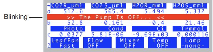
While in New Measurements mode, there are a few situations that will cause OPEN to alert you to possible problems. Experiment #2 illustrated two. The complete list of possible causes is in New Measurements Mode Warning Messages. When such a situation occurs, a warning message is displayed on the middle label line on the display, as illustrated in Figure 3‑29.
If you wish to disregard the displayed message and get it out of the way, press ctrl Z to turn it off (hold the ctrl key down and press Z). Note that this is a toggle: if you press ctrl Z again, the message will re-appear. Also, note that each time you re-enter New Measurements mode, OPEN resets this flag, so that warnings will again be displayed.
Dynamic Response of Humidity Control
We’ll do one more humidity control experiment, but this time track what is happening using real time graphics. Part A of the experiment defines the graphics display, and part B does the work.
Experiment #3 Watching the Dynamic Response of Humidity Control
Part A: Set up an RTG display for RH_S and Flow
The editor we’ll be using is fully described in Real Time Graphics on page 6-14 in the instruction manual. But for now, just follow along and you’ll get the job done.
- Select a Graphics Display
- Press 4 to view the Real Time Graphics control keys, then press f3 (View Graph). Find an unused graphics display (F in our example).
- Launch the Plot Editor
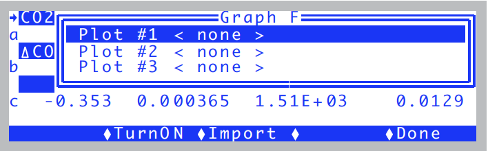
- Press 2 to bring up the function key labels, then press f4 (EDIT). The display will look like this:
- Enable Plot #1
- Press f2 (TurnON). When offered a choice between StripChart and XYChart, press S (or f1) for StripChart.
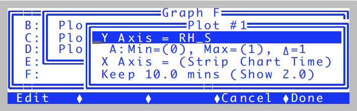
- Define the StripChart
- The Plot Editor for StripCharts will appear (Figure 3‑31). The top line, "Y Axis =" shows the variable to be plotted, and presently there is none defined.
- Select RH_S
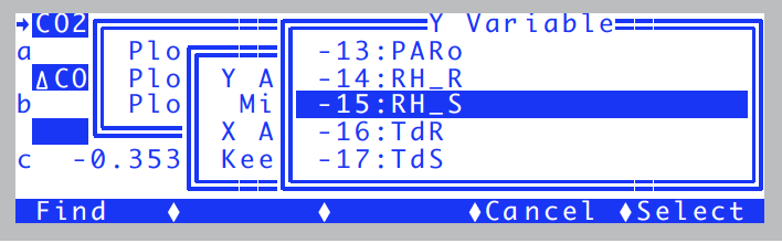
- With the top line (
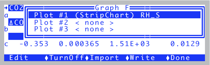
Y Axis =) line highlighted, press f1 (edit). A list of variables will appear. Page down (press pgdn) a few times until you get to the line that says-15:RH_Sand select it by pressing f5 (Select) or enter (Figure 3‑32). - Then press f5 (Done) to end the plot definition. The display should appear as in Figure 3‑33.
- Add a Flow Plot
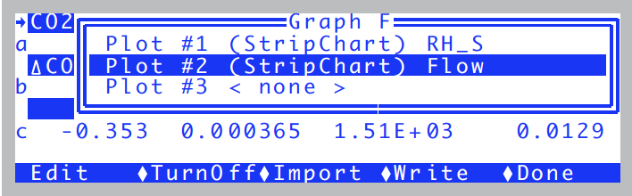
- Press ▼ to highlight Plot#2, and press f2 (TurnOn). Select StripChart. Then edit the Y Axis entry and pick flow rate, ("
-7:Flow"). Press Done (f5). - Exit the Graph F editor
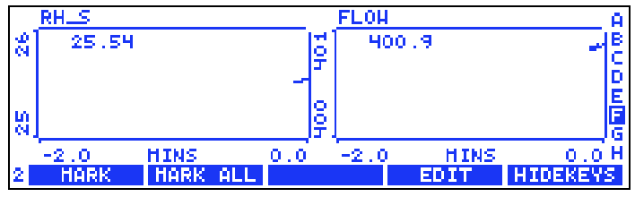
- Press Done (f5). You will go back to viewing Graph F, and it will start operating (Figure 3‑35).
- Press escape or ] to return to text mode.
Part B: Do the Test
We’ll now change the input humidity from dry to ambient and back, and watch how the flow rate adjusts.
- Fixed Flow at 400, Desiccant mid-range. Pick a target.
- Press f2 (level 2), set for flow rate, then t 400 enter. Note the RH value (RH_S_%, line b). This value will be the target in the next step.
- Constant RH
- Switch to Relative Humidity mode, enter the current RH_S_% value as the target (f2, pick Relative Humidity, then t c enter).
- View the Graph
- Press ].
- Turn the desiccant to full bypass
- Wetter air will enter the chamber, so flow must increase to maintain the target humidity.
- Wait about 15 or 20 seconds, turn to full scrub
- The flow drops to a new value, but humidity stays the same. You should see something like Figure 3‑36
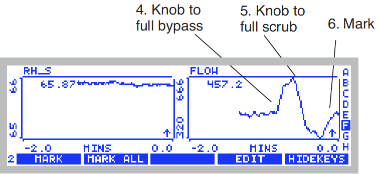
- Mark the Plot
- Press f1 (MARK). This will mark on the plots the time we changed response time (next step).
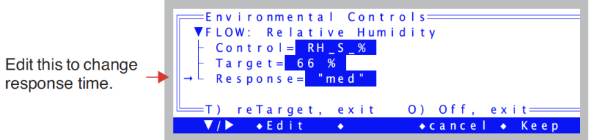
- Change to medium response.
- Press ] to stop viewing the graph. At level 2, press f2, then change the response to medium. Then press Keep. Resume watching the graph by ].
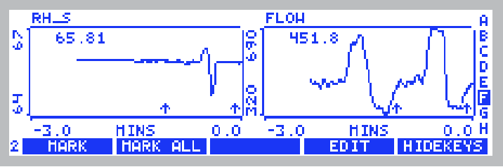
- Full bypass, Full Scrub, Mark
- Repeat the sequence: Full bypass, wait 10 secs. Full scrub, wait 10 secs, then back to middle, wait 10 secs, and mark (Figure 3‑37).
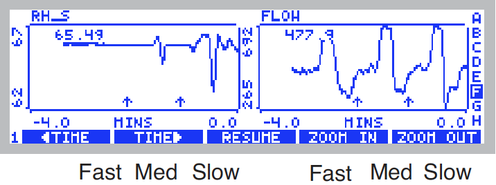
- Once more at slow response.
- Change to slow response (], f2, change response to slow, keep, ]). After you’ve scrubbed and bypassed, you should see something like Figure 3‑38.
Points to Remember
There is a control trade-off: stable humidity and unstable flow vs. unstable humidity and stable flow. (For details and suggestions, see the discussion under Humidity Time Response on page 7-12 in the instruction manual.)
Typically, you will be best served by operating with RSPNS=fast for the “tightest” humidity control. RSPNS=med will have reduced system noise, however.
CO2 Control - Without a 6400-01 Mixer
In the absence of a 6400-01 CO2 Mixer, the LI-6400’s means of controlling CO2 is limited to the soda lime adjustment knob. The following experiment illustrates how this works.
Experiment #4 Adjusting the Soda Lime
For this experiment, the chamber should be empty and closed.
- Fixed flow of 500 μmol s-1
- Press 2, f2, flow rate, t 500 enter.
- Soda lime full scrub, desiccant full bypass
- This will provide incoming air that is free of CO2.
- Note the reference and sample CO2
- They should both be near zero, and stable. Photosynthesis (Photo, line c) should be stable. (If Photo not zero, it’s because the sample and reference IRGAs aren’t reading the same thing. Matching the Analyzers, will take care of that, but we’ll ignore it for now.)
- Desiccant full scrub.
- Watch CO2R_μml or CO2S_μml, and note the burst. That’s CO2 that flushed out of the desiccant tube; the desiccant buffers CO2 chemically as well as volumetrically.
- Soda lime full bypass, desiccant full bypass
- Now we’ll let ambient air into the chamber. Watch how unstable photosynthesis becomes.
- Unlike Step 3 when we were scrubbing all the CO2 from the air, the reference and sample CO2 are now fluctuating as unmodified, ambient air enters the system. If you want to see real instability, breathe near the air inlet on the right side of the console, and watch what happens to photosynthesis.
Points to Remember
- The soda lime scrub setting controls reference CO2, from ambient down to zero.
- You’ll need a buffer volume to make stable measurements. See Air Supply Considerations.
- The desiccant buffers CO2.
CO2 Control - With a 6400-01 Mixer
Life is simpler with a CO2 mixer, as the following will demonstrate.
Experiment #5 Using the CO2 Mixer
Prepare the 6400-01 (see 6400-01 CO2 Injector Installation), and install a 12 gram CO2 cartridge.
- Set the flow control for a fixed flow at 500 μmol s-1.
- Press 2, f2, F, 500 enter.
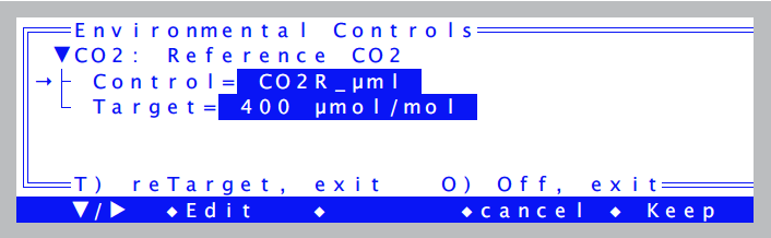
- Turn on mixer and set a 400 μmol mol-1 reference target.
- Press f3 and make the stream look like this,
- then press f5 (Keep). Set the soda lime to full scrub.
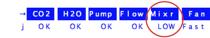
- Put status line J on middle line
- The mixer status (Mixr) can show OK, Low, or High.
- If you’ve just installed the CO2 cartridge, Mixr will probably show Low (not enough CO2 pressure). Eventually (after 2 or 3 minutes), it should show OK, and the CO2R_μml value (line a) should be close to 400, the target.
- Once CO2R_μml is stable, change target to 200 μmol mol-1
- Press f3, t, 200, enter. Notice how much faster CO2R_μml drops than rises. It may overshoot or undershoot the target value, but will correct itself eventually. Calibrating the mixer (we skipped it, but it’s described on page 18-25 in the instruction manual) can improve this performance.
- Once CO2R_μml is stable, change to 20 μmol mol-1
- Press f3, t, 20, enter. CO2R_μml won’t make it to 20, but will probably stabilize between 30 and 50 μmol mol-1. Notice the Mixer status (Mixr on line j) will be High.
- Change to 2000 μmol mol-1
- Press f3, t, 2000, enter. It will take a few minutes to reach this, and Mixr will be Low for much of this time. When CO2R_μml finally does reach 2000 μmol mol-1, it should be fairly stable.
- Change to 400 μmol mol-1
- Press f3, t, 400, enter. CO2R_μml should drop to 400 μmol mol-1 much faster than it rose to 2000 μmol mol-1.
Points to Remember
- Soda lime must remain on full scrub when using the mixer
- The lowest stable value is typically between 30 and 50 μmol mol-1. See (Support: LI-6400/XT Portable Photosynthesis System)
- Mixer adjusts faster when lowering the concentration, than raising it.
Experiment #6 Dynamic Response of the CO2 Mixer
We’ll need StripCharts for CO2R and CO2S (where we’re headed is Figure 3‑39). They are likely already defined, on Graph B. If not, set them up yourself, following the example in Part A: Set up an RTG display for RH_S and Flow. (Hint: CO2R and CO2S have ID numbers -1 and -2 in the list of variables that appears when you edit the Y axis.)
- Close the empty chamber
- It’s another no-leaf experiment.
- Fixed flow at 500 μmol s-1
- Press 2, f2, flow rate, t, 500, enter.
- Set the mixer for a 400 μmol mol-1 reference target
- Press f3, reference, t, 400, enter. Watch the graph (]).
- After 1 minute, change reference target to 900 μmol mol-1.
- When the CO2S curve flattens out, press ], f3, t, 900, enter. Resume watching the graph (]).
- After 1 minute, change the reference target to 100 μmol mol-1.
- When the CO2S curve flattens out, press ], f3, t, 100, enter, followed by ] to continue viewing the graph.
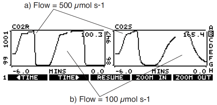
- Redo Steps 4 through 5 with Flow = 100.
- Reduce the flow rate, and repeat the cycle. Note the slower response of the sample cell, and the faster response of the reference cell.
Your results should be similar to Figure 3‑39.
Points to Remember
Controlling on reference concentration is faster than controlling on sample concentration, for 3 reasons:
- The larger volume of the sample cell / leaf chamber.
- Flow changes when controlling constant humidity.
- Possible photosynthetic rate changes.
Temperature Control
Temperature control has two target options: a constant block temperature (the block is the metal block that encompasses the sample and reference cells of the IRGA), or constant leaf temperature. Temperature Control on page 7-18 in the instruction manual has details, but the next two experiments illustrate the differences.
We’ll use StripCharts for both of these experiments, monitoring block temperature, air temperature in the sample cell, and leaf temperature. Graph D should already be configured for this, but if not, the ID numbers for our three temperatures are -8, -9, and -10.
Note: You can extend the temperature range of the coolers by using the expanded temperature range control kit 6400-88.
Experiment #7 Controlling on Block Temperature
This is the more direct and stable of the temperature control options.
- View the temperature line.
- Display line h of the default display map has block, air, and leaf temperatures.
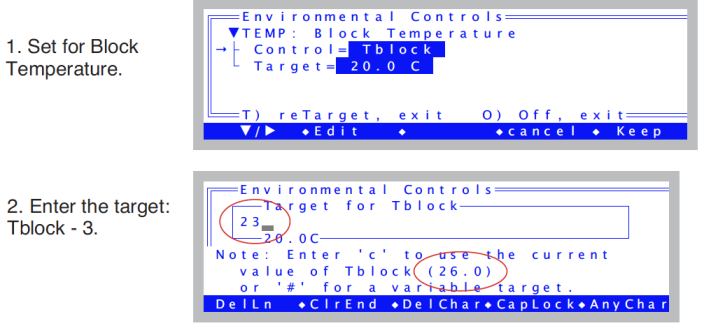
- Set block target to 3 °C cooler than current value.
- Press f4 (level 2), block temp, t <value- 3> enter (where value is the block temperature from Step 1).
- Note the temperature gradient
- You should see that Tblock < Tair < Tleaf.
- Now make the target 3 °C warmer than ambient
- Press f4 <value + 3> enter . The block temperature will rise a bit faster to this new target. Heating is always more efficient than cooling.
- Note the temperature gradient
- You should see that Tblock > Tair > Tleaf.
- Return to ambient
- Set the block temperature back to the starting point.
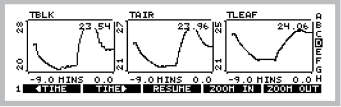
The graph for this experiment might look like Figure 3‑40.
Points to Remember
- Controlling on block temperature is slow but steady.
- Limit of control is generally within 7 °C of ambient.
- The further Tblock is from ambient, the larger the temperature gradient through the leaf chamber and IRGA.
Experiment #8 Controlling on Leaf Temperature
For this experiment you’ll need slightly damp filter (or towel) paper to act like a leaf.
- Observe Tleaf
- Tleaf°C is on display line h.
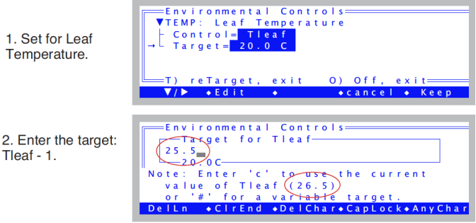
- Control leaf temperature to 1°C cooler than it’s present value
- Press f4, level 2, leaf temp, t, <value - 1> enter.
- Watch what the block temperature does
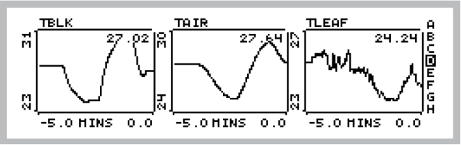
- Press ] to view the strip charts (Figure 3‑41a). The block temperature will drop in discrete increments as the control algorithm works to get the leaf temperature down to where it belongs.
- Now add 1 degree to the target leaf temperature
- Press ] to get back to text mode, then f4, t, < value + 1> enter. Then ] to view the strip charts (Figure 3‑41b).
Points to Remember
- Block temperature will warm or cool as needed in its efforts to control leaf temperature.
- Leaf temperature control is not as fast or stable as block temperature control, since the mechanism is to control the temperature of the air that is blowing by the leaf, whereas the real factors driving leaf temperature include radiation balance and physiology.
Lamp Control
If the light source is attached (the procedure is described on Attaching the LED Light Source), but OPEN is not presently configured to use it2, then do the following:
To configure OPEN for a controllable light source:
- Access the system configuration
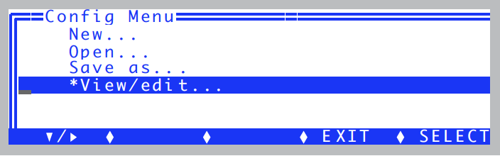
- This is done by
Config Menu|View/edit. Press escape to leave New Measurements mode. In OPEN’s main screen, press f2 (Config Menu), then highlight the entry “View/edit...”, and press enter. - Attach a Light Source
- Use whatever you have available: 6400-02B LED, 6400-18 RGB, or 6400-40 LCF.
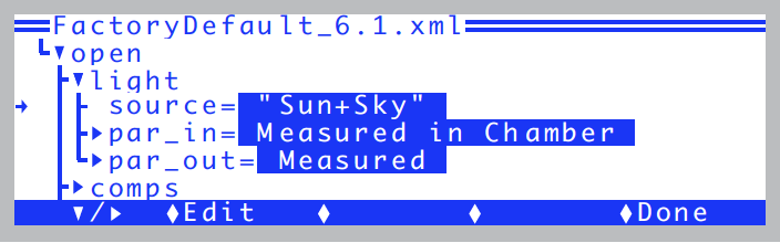
- Navigate to the open - light - source node
- (Remember f1 will open closed nodes.)
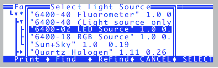
- Press f2 (Edit) and pick a source
- A menu of possible light sources appears. Choose the appropriate 6400-02, 6400-18, or 6400-40 entry, and press enter.
- Return to New Measurements Mode
- Press f5 (Done), to return to the Config Menu, then escape to return to OPEN’s main screen, then f4 (New Msmnts).
The lamp control is the most straight-forward of all the control algorithms. The feedback is immediate, since there is a sensor located in the light source measuring its output, and there is no other mechanism (such as flow rate) that will interfere with the light value3.
Experiment #9 Simple Lamp Control
- Close the chamber, no leaf
- Monitor in-chamber PAR on the display
- Press G. The in-chamber PAR value is ParIn_μm on display line g.
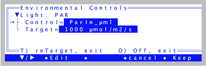
- Set the lamp for PAR, 1000 μmol m-2 s-1.
- Press f5 (level 2), PAR, t, 1000, enter.
- Watch ParIn_μm
- The ParIn_μm value will go to a value fairly close to the target, and then a few seconds later shift to the exact target value.
- Open the chamber
- When you open the chamber the ParIn_μm value will drop about 10% due to the sudden decrease in reflectance. Note: this is NOT true for the 6400-18 RGB. It has some on-board circuitry that keeps it locked on to the target when you change the amount of light reflecting back into the lamp (Internal Feedback on page 8-18 in the instruction manual).
- Watch ParIn adjust
- After several seconds, the ParIn_μm value will increase to the target, as the light source brightens to make up for the decreased reflectance.
- Turn the lamp off.
Points to Remember
- As with the other controls, the light source is active, adjusting for changing conditions in the leaf chamber or light source itself.
- The light source control uses a “first guess” when given a target. If the guess isn’t on target, it adjusts itself to the correct value. There is a calibration routine (in the Calib Menu) that can be run that generates data for these first guesses. This is described on page 6400-02(B) LED Source (for the light source) or Calibrate... (for the fluorometer).
Control Summary
Even though the four control areas that we’ve just explored have very differing hardware (a pump and/or proportioning valve for humidity control, LEDs for light control, etc.), they have common interfaces and logic. In fact, this control software offers some powerful features that our tour did not touch upon. Chapter 7 provides a more thorough discussion of these controls, their options and limitations. At some point in your experience with the LI-6400, you should take time to read this material, and acquaint yourself more fully with these tools.