Other software settings

This section describes features that have not been described elsewhere.

Settings

Under Settings, you can set the instrument time, network configuration, send commands, change the chopper housing temperature set point, and integrate CO₂ measurements.

Time

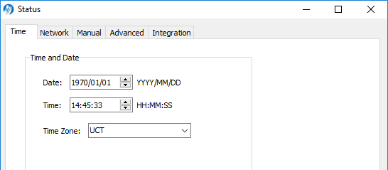
This is where you set the instrument time and date. The instrument clock uses the Precision Time Protocol (PTP) time keeping system. PTP is a high precision time synchronization protocol for networked devices. Devices controlled with PTP can maintain accuracy in the sub-microsecond range with a sufficiently accurate master clock. PTP is defined in the IEEE 1588-2002 and 1588-2008 standards, entitled “Standards for Precision Clock Synchronization Protocol for Networked Measurement and Control Systems.” A detailed summary of IEEE-1588 is available at www.ieee1588.com. Full documentation is available for purchase from the Institute of Electrical and Electronics Engineers (IEEE) at www.ieee.org.

The basic principle behind PTP is that the best time keeping can be accomplished with multiple networked devices by synchronizing all device clocks to the most precise clock on the network. Each clock on the network has a rating that indicates its relative accuracy. The IEEE 1588 protocol specifies the use of a Best Master Clock algorithm to determine which clock on the network is the most accurate. On a network, the most accurate clock becomes the master clock and all other clocks sync to the master clock.

The software implementation of PTP provides accuracy in the 10 microsecond range. When used with the SmartFlux System, the GPS clocks will become the master clock for the system.

About time keeping

The LI-7500A/RS/DS and LI-7200/RS are network-based instruments and it is possible for multiple users to log data from a single instrument over multiple TCP/IP connections. Consequently, the analyzer uses Coordinated Universal Time (UTC) for its onboard timekeeping tasks. The default time stamp is therefore UTC based, but local time can be set, if desired.

Generally, we recommend that the system synchronizes its time to the GPS clocks. The instrument uses a time zone database that includes local time zones that are kept as constant offset from UTC. These time zones are listed as ‘Etc/GMT’ + offset. However, these time zone names beginning with ‘Etc/GMT’ have their sign reversed from what is commonly used. Thus, zones west of GMT have a positive sign, and those east have a negative sign. For example, US/Central Standard Time is 6 hours behind GMT, and in the database this time zone is listed as ‘Etc/GMT-6’.

Unix time is the number of seconds elapsed since the Unix epoch of 00:00 Coordinated Universal Time (UTC) January 1, 1970 (or 1970-01-01T00:00:0Z ISO 8601). For example, the time stamp 1262884605 translates to 01/07/2010 at 05:16:45 UTC. The date and time are converted to a conventional display format (YYYY-MM-DD; HH:MM:SS) and adjusted based on the time zone setting that you select.

The time stamp in each file header shows the instrument time and time zone.

Setting the clock

1. Connect to the gas analyzer.
2. Open the Settings window.
3. Set the Clock Sync (PTP).
4. Choose your time zone.
5. Click Apply or OK.

The PTP clock settings available are:

• Off: Turns PTP time keeping system off. Instrument time will be determined by the Date and Time set by the user, even if there is a better clock on the network.
• Automatic: The gas analyzer searches the network and syncs to the most accurate clock using the Best Master Clock algorithm (could be the gas analyzer). This setting should be used in most circumstances.
• Slave Only: The gas analyzer always syncs to another clock. It will search the network and synchronize to the best clock.
• Preferred: The gas analyzer uses its own internal clock unless it finds a better clock on the network.

Network

The instrument name is given in the Connect window and Settings > Network window. You can change this name in Settings > Network. The name can include upper and lower case letters (A to Z; a to z), numbers (0 to 9), dash (-), and period (.). Other characters are invalid and will cause communication errors with the system.

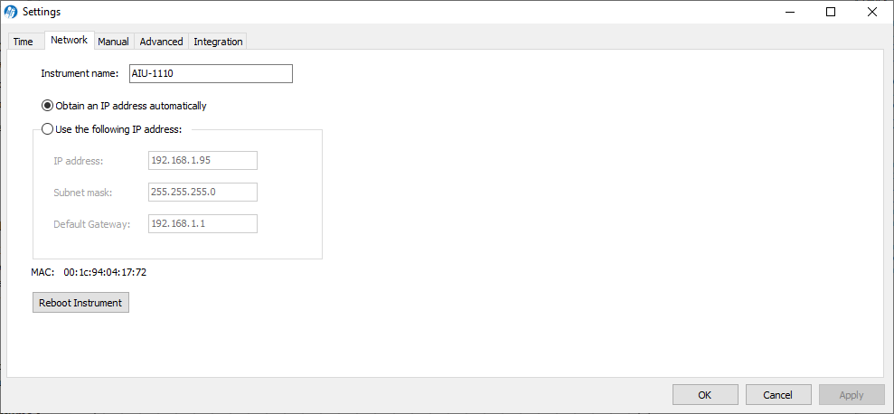
The IP address (Internet Protocol) is a numerical identifier that is assigned to devices participating in a computer network. In many cases this address is assigned automatically (Dynamic IP address). In other cases, your network administrator may assign a permanent address (Static IP address) that can be entered manually.

With Obtain an IP address automatically selected, the IP address, Subnet mask, and Default Gateway fields are filled in automatically; if you choose to enter the IP address manually, the address fields are editable.

The Subnet mask is a set of 4 octets used to separate an IP address into two parts; the network address and the host address. The Gateway is a node that routes traffic to another network.

Manual addressing

You can connect to an instrument by manually enter the IPv4 Address or Hostname of the instrument. The IP address can be set automatically by a network or assigned manually in Settings > Network > Use the following IP address. If IPv6 (Internet Protocol version 6) addressing is available on the network and enabled on the computer, the instrument’s IPv6 address is displayed as well.

Both the LI-7500A/RS/DS and LI-7200/RS use the Port number 7200 for Ethernet communications. Therefore, when connecting to the instrument on a network you will enter the IP address of the instrument and port 7200 in the connection window of the software to initiate communication. You can select the instrument from the list of instruments on the same network as your computer or connect your computer directly to the instrument Ethernet port.

Port forwarding

In some network setups it may be necessary to forward communication traffic on a port from a public IP address to a private IP address to gain access to an instrument. For example, assume you have an analyzer installed in the field and the instrument is connected to a wireless gateway such as a cellular modem. The instrument will acquire a private IP address from the cellular modem, but this address is only visible to nodes on the private network. On the other hand, the cellular modem is assigned a public IP address that can be accessed from any node on the Internet. For this discussion let’s assume the public address is 166.66.77.88. In order to connect to the instrument in the private network, a port forwarding rule must be created in the cellular modem to “forward” all communications on port 7200 coming into the modem to the private IP address of the instrument.

Instrument	Example Public IP	Public Port	Private IP	Private Port
1	166.66.77.88	7200	192.168.13.201	7200

The public port number should be changed when there is more than one LI-7500A/RS/DS or LI-7200/RS instrument in the private network. In this case, to connect to each instrument, two port forwarding rules must be set up, similar to that shown below.

Instrument	Example Public IP	Public Port	Private IP	Private Port
1	166.66.77.88	7201	192.168.13.201	7200
2	166.66.77.88	7202	192.168.13.202	7200

You can run multiple LI-7500A/RS/DS or LI-7200/RS software sessions at the same time to communicate with different analyzers. Simply double-click on the software icon to open another session, and connect to a different instrument.

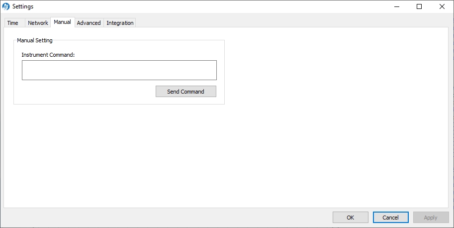
Manual

A command line field is present that allows you to send a command to the instrument. This can be useful for diagnosing problems, as a LI-COR technician can gauge the instrument’s response to given commands, and determine if the instrument is functioning properly. Contact LI-COR technical support for details on the grammar.

Advanced—Chopper housing temperature

The chopper motor housing temperature can be set to a lower operating temperature (5 °C) in winter to reduce power consumption and minimize heating by the electronics. We recommend changing the setting only when the average ambient temperature drops below 5 °C. You can change the setting back to 30 °C when the average ambient temperature is above 5 °C. Note, however, that the instrument will still function properly when the chopper motor housing temperature is set to 30 °C, even when temperatures are below 5 °C.

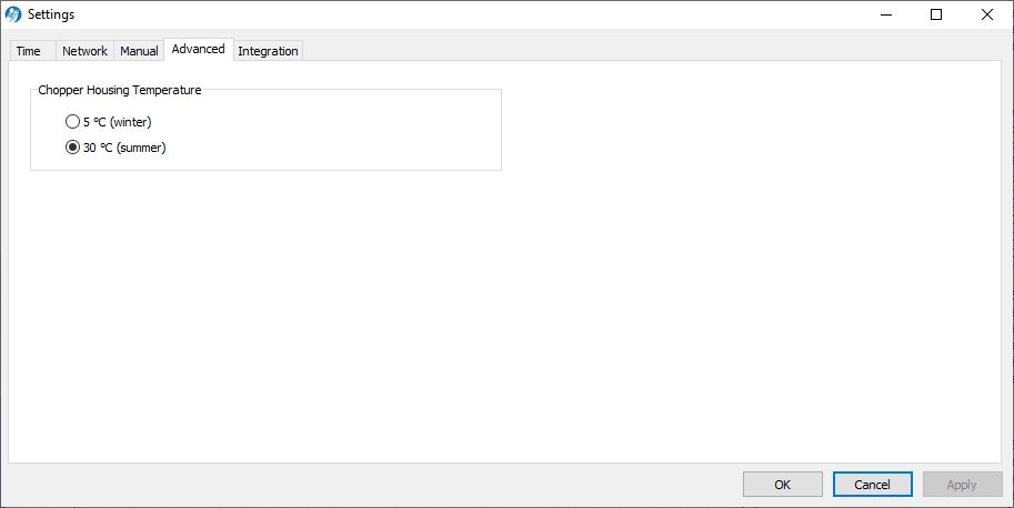
Do not set the chopper housing temperature to 5 °C when ambient temperatures are above 5 °C, however, as the instrument will not function properly.

Important: When changing between winter and summer settings, you will need to perform a zero and dual span calibration.

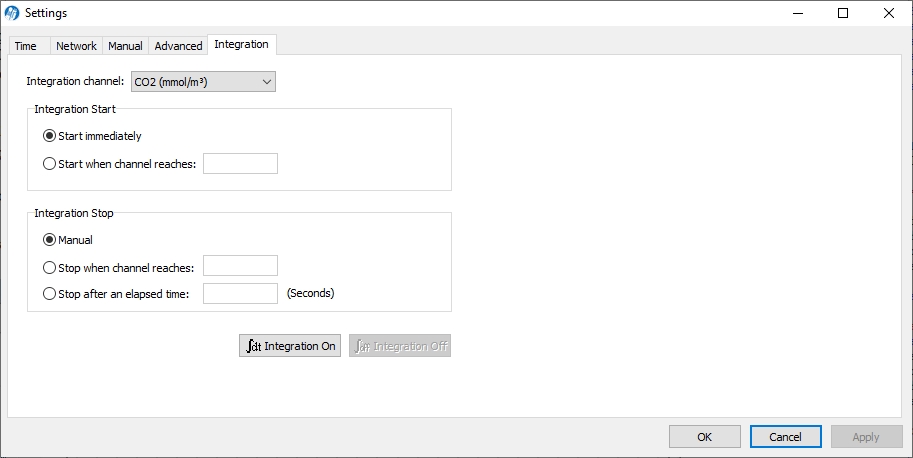
Integration

Allows for the setup of an integration function using a selected CO₂ source (mmol/m³, µmol/mol, or dry µmol/mol). The integrated value selected can be viewed as a data source in the main software window (choose Integral in the Data Items list). To integrate a CO₂ source:

1. Choose a source to be integrated from the Integration Channel list.
2. Choose the method to start the integration; immediately, or using a threshold value.
3. Choose the method to stop the integration; manually, with a threshold value, or after a user-entered elapsed time has expired.
4. Enter the threshold value for the start or stop (or both) of the integration, if either was chosen in Steps 2 or 3 above.
5. Click on the Apply button.
6. If Start Immediately was chosen for the Start Time, the integration function is started and/or stopped manually by clicking the òdt Integration On or òdt Integration Off buttons (available on the dashboard, as well).



7. Example: Start integrating CO₂ (µmol/mol) after it reaches a value of 500 µmol mol^-1, and continue integrating for 5 minutes.
6. Choose CO2 (µmol/m³) from the Integration Channel list.
7. Click Start when channel reaches button and enter 500 in the text entry field.
8. Click the Stop after an elapsed time button and enter 300 (seconds) in the text entry field.
9. Click Apply.
10. Click the òdt Integration On button. Click OK to dismiss the dialog.

The integration result (area under the curve) can be viewed in the dashboard.

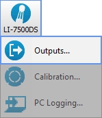
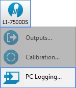
Menu overview

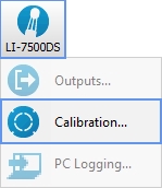
The LI-7500DS menu provides access to Outputs... settings, Calibration..., and PC Logging... settings.

Outputs

Two options are available under the outputs tab: Setup, where you set the bandwidth, and Ethernet, where you configure some optional output settings.

Setup

The Setup tab presents Bandwidth and Ethernet output options.

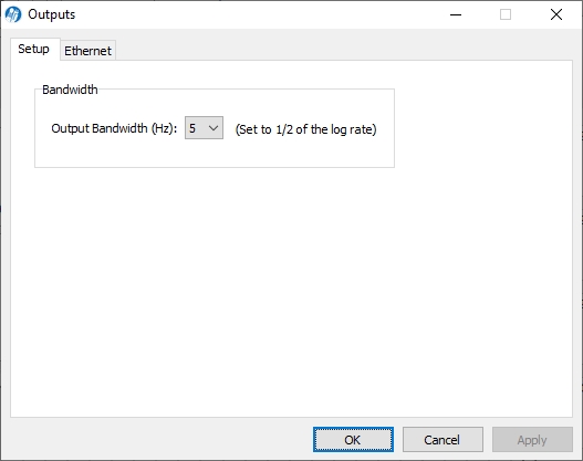
Output bandwidth

Bandwidth (5, 10 or 20 Hz) determines the signal averaging done by the digital filter. To avoid aliasing (only a concern for co-spectra, not for fluxes), one should sample the gas analyzer at a frequency greater than or equal to 2 times the bandwidth. Thus, if you are sampling at 10 Hz, the bandwidth is 5 Hz.

Bandwidth is the frequency at which the indicated amplitude is 0.707 of the real amplitude (Figure 10‑1).

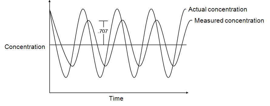
Bandwidth is a useful indicator for characterizing real-world behavior in which there are fluctuating gas concentrations. Given a sinusoidal oscillation of concentration, the instrument's ability to measure the full oscillation amplitude diminishes as the oscillation frequency increases.

Ethernet output

The Ethernet tab is used to set the instrument's Ethernet output. After configuration, click Apply and the analyzer will begin to send data out the Ethernet port according to these parameters.

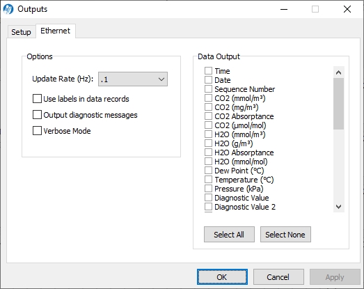
Use the Update Rate menu to select from 0.1, 0.2, 0.5, 0, 1, 2, 5, 10, or 20 Hz.

Under Options, you can choose whether or not to output labels with each data record, whether to output diagnostic text records, and whether to use verbose mode. An example of a data record sent with and without labels is shown below.

Data format with labels:

Data format without labels

Under Data Output, select the data records that you want to output; click Select All to choose all, or Select None to disable all checked values.

The data items available for display given in Support: LI-7500DS and SmartFlux® 3 System.

Calibration window

The Calibration window is where you set the zero and span of the instrument. There are entry fields to set the target values for the span gases used to set the span of the instrument; CO₂ span gas target values are in ppm, and H₂O span gas target values are entered in °C dewpoint. The Zero and Span tabs also provide information about the stability of the gas flowing through the optical path:

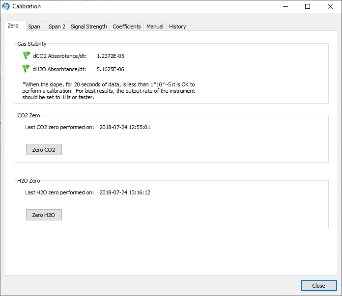
• A green flag indicates that it is OK to perform the calibration
• A red ‘X’ indicates that it is not OK to perform the calibration; wait until the red ‘X’ changes to a green flag before performing the calibration.

Zero, Span, and Span 2 tabs

These tabs are where you interact with the software when you set the instrument calibration. They are described in User calibration.

Signal strength tab

The Signal Strength tab has a button labeled Reset Signal Strength that you can click if you’ve decided your instrument optics are as clean as you can reasonably make them, and you want to reset the signal strength to 100.

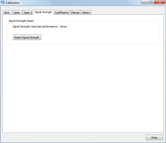
See CO2 signal strength for more information.

Coefficients tab

The Coefficients tab displays factory-determined calibration coefficients, a factor for correcting CO₂ measurements for band broadening due to the presence of water vapor (A), and a zero drift correction factor (Z). The coefficient shown as XS (cross sensitivity) compensates for slight cross sensitivity between CO₂ and H₂O signals absorbed by the detector.

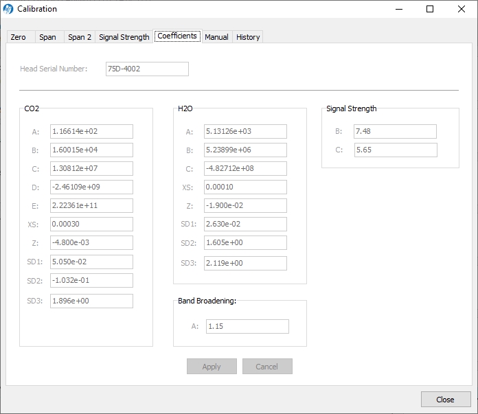
The calibration coefficients, XS, and Z values are unique to each sensor head, and may be found on the calibration sheet shipped from the factory. The Band Broadening coefficient is 1.15 for all sensor heads.

Caution: To avoid undesirable changes to the instrument performance, do not edit values in this window. Click Cancel to avoid any undesirable changes.

The Head Serial Number displays the serial number of the sensor head that is associated with the coefficients.

Manual tab

The Manual tab displays current values for CO₂ and H₂O zero and span; after performing a zero and span calibration, these values should be near 1 (zero is typically between 0.8 and 1.2, and span is typically between 0.8 and 1.2; Z_wo and Z_co,. Span 2 values will be near zero.

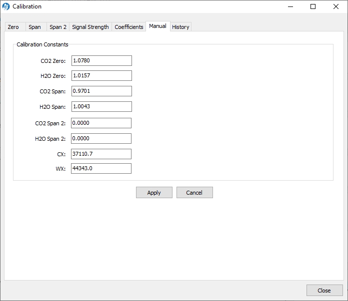
We recommend that you track the zero values over time as you re-zero the instrument. As the internal chemicals lose their effectiveness, this value will increase. The CO₂ zero drift is also somewhat temperature dependent.

In most cases you will never need to manually edit these values. If, for some reason, the instrument calibration becomes unstable (e.g., you accidentally zeroed or spanned the instrument with the wrong gas), you can manually enter a value of 1 for each of these parameters (and zero for Span 2 values), and click Apply. This will return the instrument to a more normal state, after which you can perform zero and span calibrations again. Alternatively, if you have performed at least one previous (successful) calibration, you can restore those values using the History tab.

History tab

The History tab displays a list of previous calibration backup files generated during a zero and/or span calibration of the instrument (when used with the same computer used to connect to the instrument). You can click on any previous calibration in the list to view the details; you can also restore the values from a previous calibration by choosing a file in the list and clicking the Restore button. Click Delete to permanently remove calibration files from the list stored on the computer.

PC logging

The PC Logging window is used to configure the data output parameters used while the LI-7500A/RS/DS or LI-7200/RS Windows software is active. Data are logged to a file on your computer. You can specify the destination file, update rate, file duration, comments, and values to be logged.

Data can be logged at up to 20 Hz. These files can be split into smaller files, at 15, 30, 60 minutes, or 1.5, 2, 4, or 24 hour intervals. The files are split based on fractions of the hour as measured by the system clock. Thus, if you choose to split the files at 15 minute intervals and start logging at 10:22, the file will be split at 10:30, 10:45, 11:00, etc.

Note: File compression and metadata information are not available when logging to a PC; these options are available only when logging to the USB drive.

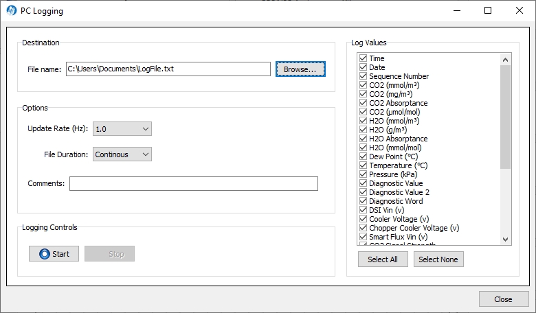
Under Log Values, select the data records that you want to output; click Select All to choose all variables.

Click Start to begin logging data and Stop to quit logging.

Diagnostics

The Diagnostics page allows you to view the current operational state of the instrument, including current software versions, diagnostic flags, optical bench properties, and technician test point values.

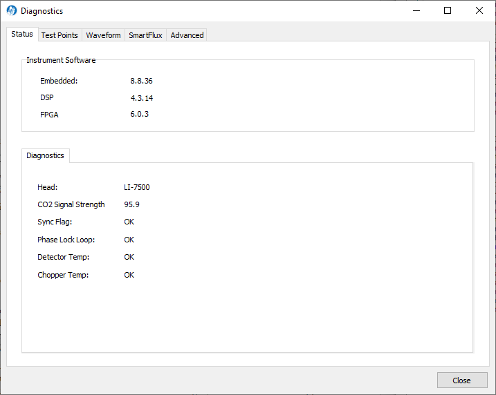
Status tab

Status indicators provide diagnostic information about the instrument.

GHG Embedded: Firmware version running on the SmartFlux System. Formerly known as SmartFlux 3 Embedded.

DSI Embedded: Firmware version running on the LI-7500DS DSI box.

LI-7500DS Diagnostics tab: If any of these are in a not OK state that cannot be resolved by cleaning the optics, contact technical support.

SmartFlux Vin (V): The voltage at the SmartFlux System.

DSI Vin (V): The voltage at the LI-7500DS DSI box.

The remaining diagnostic indicators show whether things are performing as expected. If any of these are unable to resolve an error state (not OK), call technical support to troubleshoot the issue.

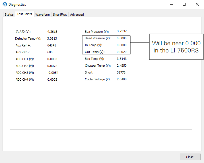
Test point values

The Test Points tab displays voltages and raw counts of a variety of diagnostic test points. Though primarily for LI-COR technician reference, values outside of the normal range may give you an indication of where problems may be originating.

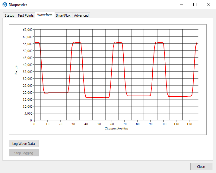
Waveform

The Waveform tab displays the current state of the analyzer’s chopping shutter disk. Though primarily for LI-COR technician reference, if problems are encountered, it may be useful to log the waveform data for troubleshooting purposes. Waveform data can only be logged when the Diagnostics window is open.

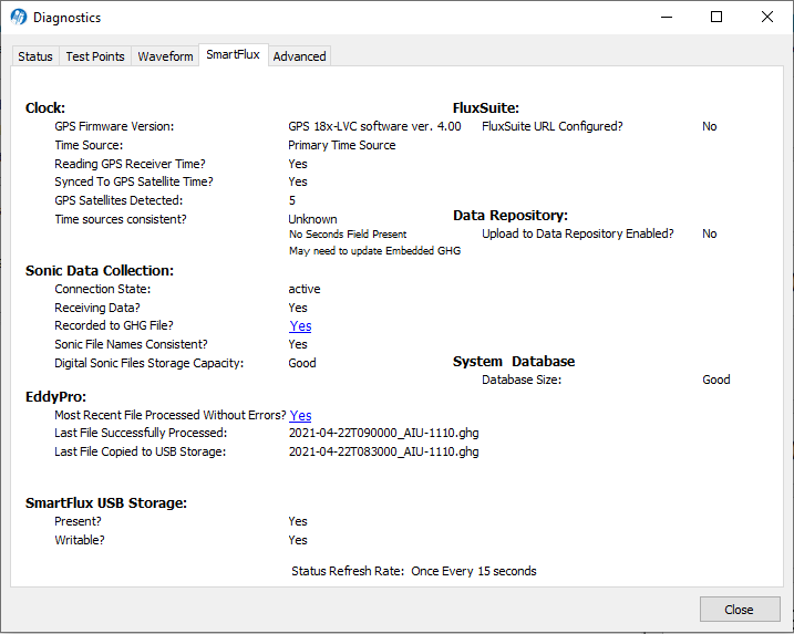
SmartFlux

SmartFlux System diagnostics are supported by the combined release of win-GHG interface software v8.8.36 and SmartFlux 2/3 System embedded firmware v2.2.50. This feature serves to summarize the system performance by providing status indicators for components and configurations, allowing you to evaluate the system at a glance. Diagnostics are under Diagnostics > SmartFlux tab.

Advanced

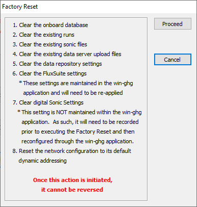
The Diagnostics > Advanced tab provides several maintenance and recovery options. These options should be used only after consultation with LI-COR technical support or careful consideration, as all of theses actions except for Reboot SmartFlux will permanently remove data from the device. Once data are removed from the USB device, they cannot be recovered. These actions are performed only on the SmartFlux 2/3 device. Each of these buttons requires confirmation after being clicked.

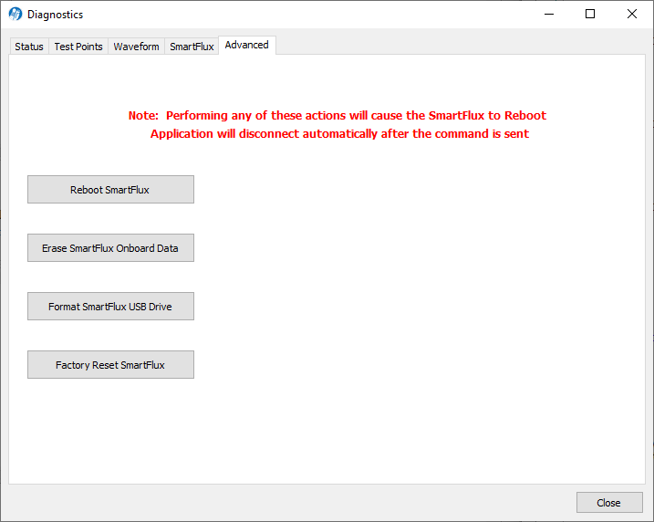
Important: After clicking any of these buttons, the desktop PC application will disconnect from the instrument. This is confirmation that the command was sent successfully. Do not disconnect manually after clicking; doing so may prevent the command from being sent.

• Reboot SmartFlux will simply restart the device. Use this if the SmartFlux System is not responding to configuration changes or is not communicating properly. This may cause the Win-GHG application to disconnect (for the SmartFlux 3 system).
• Erase SmartFlux Onboard Data will clear the internal database, raw data files, results files, and files set for upload from the memory of the SmartFlux System. Use this when the SmartFlux internal database is too large or the internal memory has filled up.
• Format SmartFlux USB Drive will clear data from the USB drive in the SmartFlux System. Use this when having problems with USB data logging or if manually deleting old files is taking too long.
• Factory Reset SmartFlux This performs all the items listed under Erase SmartFlux Onboard Data and also removes user configuration such as sonic, and networking. Use this in very rare case where the SmartFlux is malfunctioning and is not able to be configured. The application requires you to wait 15 seconds to contemplate the choice before allowing you to proceed.

Important: If you are moving the SmartFlux 2 from one IRGA to another, you must either Erase SmartFlux Onboard Data or Factory Reset SmartFlux. Use the first option is if you are simply moving the SmartFlux 2 from one IRGA to another that is using the same model of sonic anemometer. Use the second option if you are moving the SmartFlux 2 from one IRGA to another and installing a different model of sonic anemoemter.

Charting

The Chart window allows real time graphics display of one or two variables plotted against time. The Y-Axis displays the value chosen in the respective menu against time on the X-Axis.

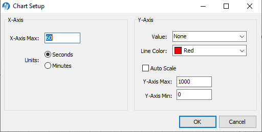
Time on the X-Axis can be displayed over user-defined values of seconds or minutes; the X-Axis Max value defines the unit of time displayed in the window before the window starts scrolling the time value off the right edge.

Choose the value for the Y-Axis Left and/or Y-Axis Right in the menu(s), and enter values for the Y-Axis maximum and minimum; choose Auto Scale if you want the chart to scale the Y-Axis automatically to keep data from scrolling off the top or bottom edges. You can also select the color of the line for both Y-Axes values.

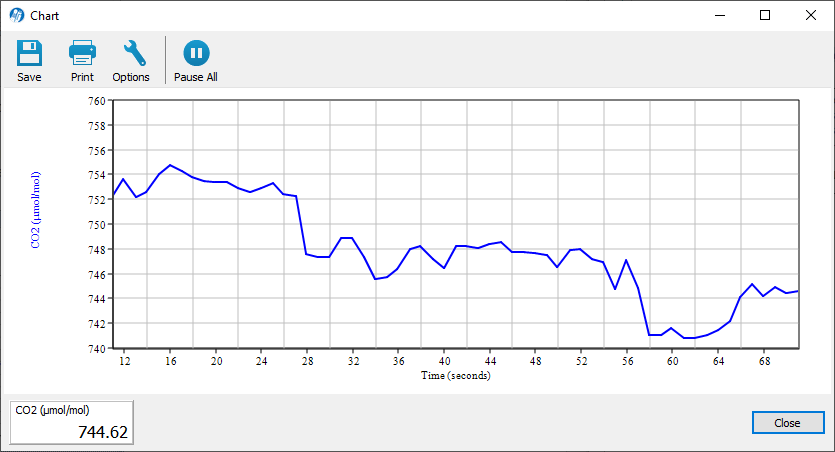
When you are finished defining the strip chart(s) parameters, click OK. A new chart window will appear. Press Pause All to temporarily stop plotting (press Pause All again to resume); press Save to save a “snapshot” of the current plot to a bitmap file; press Print to print the currently displayed chart window, or press Options to open the Chart Setup window again to make changes to the strip chart parameters.

Note: You can rescale both Y-axes of an active strip chart by right clicking on the chart, holding, and dragging up or down. You can also open as many chart windows as you want.

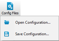
Configuration files

The instrument uses a configuration file to store parameters of the configuration, including the setup information, instrument settings, calibration coefficients, and zero and span values, and logging configuration. Unique configuration files can be set up, saved, and then re-opened to easily change your setup information.

When the software program is started for the first time, a default set of parameters is loaded, which can be modified and saved as a new configuration file with a different name. The analyzer stores its configuration so that it will power on configured just as it was when it was powered off.

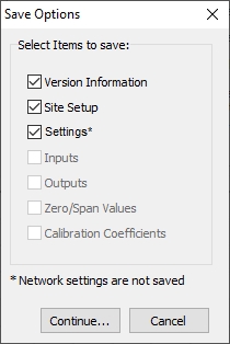
To save the current configuration, click Config File > Save Configuration. Select the items to include in the file and click Continue. Select a directory and save the file. It will have a .l7x extension.

To open an existing configuration file, click the Config Files button and select Open Configuration. Select the file and click Open. You are prompted to send the configuration to the instrument; changes are implemented in the instrument when the configuration file is loaded.