
u* Threshold Detection is a way to find the threshold at which fluxes are no longer dependent on the friction velocity. Tovi offers two distinct approaches: moving point test (MPT) and change point detection (CPD) method. This tool is applied after the first quality screening, biomet gap filling, averaging, and storage corrections have been completed.
Below we describe terms and concepts used in the u* procedure.
Bootstrap: Generally (and loosely) speaking, bootstrapping is a statistical technique to evaluate some properties of statistical estimators. For example, it allows you to evaluate the robustness of the estimator mean value. If you have a sample of anything with N = 1000 (say, the weight of people), you can compute only 1 mean value, but you don’t know much about the quality of this mean value. (For example, would it change dramatically with N different people from the sample population?) Bootstrapping is the process of “re-sampling” from your sample M times (e.g., M=100), which allows you to come up with M values of the mean, that you can use to build a distribution of the mean values, and hence get properties such as standard error, confidence interval, and more.
Bootstrapping is most useful when your estimator is a complex thing, such as the u* threshold derived with the moving point test (MPT). Tovi resamples the yearly data (u*, net ecosystem exchange, air temperature) M times, repeat the entire MPT, and come up with M different threshold values, which allows us to build a distribution of the u* threshold values and from there derive the final value as the median of that distribution.
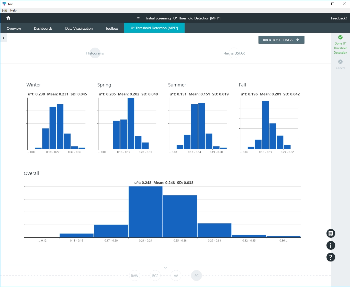
Because the MPT involves computing threshold values for each season independently, one intermediate result is the four distributions of the u* threshold (one per season), which is plotted in the histograms.
The data used to build the final histogram (the one whose median value is the final threshold) is derived by taking the maximum of the four seasonal threshold values in each bootstrap iteration, which returns M values of u*, from which we build the final histogram and derive the final u* threshold value.
Number of bootstraps: In theory, the larger the better. The compromise is between processing time and marginal returns: after a certain number of iterations the statistics don’t change significantly enough to justify additional computational cost. The implementation we have is fairly fast (being C) so we don’t perceive the cost of increasing the bootstrap iterations. 100 is ICOS and AmeriFlux default, presumably derived from years of experience.
Temperature classes: With the MPT technique we expect that after a certain u* value nightly NEE (which is essentially only respiration) does not depend on u* anymore (i.e., you reach a plateau in the plot NEE vs. u*). However, respiration depends strongly on temperature. If you put all the data together, the plateau doesn’t quite look as a plateau because of the superimposed temperature dependency (at each u*, you’ll get different NEE values due to temperature differences). If you split the data in temperature classes, instead, the plateau becomes much more visible and easier to identify with the automatic procedure.
The number of classes is a function of the amount of data. The more data, the larger the number of classes you afford. Again, the seven classes are presumably based on years of experience with the method.
For similar reasons the analysis is performed per season because respiration depends on temperature in different ways in different seasons (depending on other properties such as humidity, organic soil content and so on).
u* classes: These are used to regularize the data in the analysis of NEE vs. u*. For each u* class we take the mean u* and mean NEE, and then use this new, highly reduced dataset to do the MPT analysis. Essentially, it is a way of eliminating noise. As with air temperature, the number of classes is a function of the size of the dataset.
- Bootstrap, temperature classes, and u* classes are integer numbers because they are all "number of" something.
- The bootstrap exercise will to indicate the ideal spot for M, where the value the threshold settles and doesn’t change anymore with increasing the number of bootstrap iterations.
- The best quality assessment should be the plot NEE/u*, specifically the slope of the regression on the right of the threshold value.
Q: Is there a time you would want more (or less) temperature classes? Does it depend on the temperature ranges at your site? For example, the range of night-time temperatures during a particular season (or three months)?
A: In general yes, you would want to modulate the number of classes according to these details. But complexity needs to stop at some point. What one could do, using Tovi, is to first use the u* tool to identify which seasons contribute most to the u* threshold value. Once you know which season(s) are going to drive your threshold value computation, you can tune the settings (e.g., number temperature classes) to the data of that season(s), which you should analyze independently.
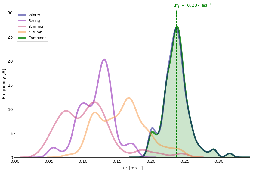
Here is a striking case of the final histogram (green) being determined almost exclusively by one season, because that season happens to give the highest u* value of all seasons almost at all bootstrap iterations. Now, you could reason in two different ways here: The season driving the computation is Winter, which happens to be the season I am least interested in. Maybe I’ll go ahead and create a new NEE variable by copying and pasting my NEE(*), but setting NEE equal to NaN for the entire winter to eliminate that season from the computation. Or, given that winter is doing virtually all the job, I will tune my settings according to the winter data.
Q: Why there are low/high tolerances for radiation, and why not for the other drivers?
A: As you are probably aware, the tolerances are intended to create ranges of the drivers’ values. For example, given T_GAP, the air temperature at the timestamp of a given flux gap, the air temperature tolerance of, say, 2.5 degrees is used to build the range [T_GAP - 2.5, T_GAP + 2.5]. This is the temperature range that flux values will be searched for in the time window (e.g., +/- 7 days around the gap), which will be then averaged to provide the flux fill value.
That said, for the special case of radiation, given the large excursion range, say 0 to 1000 W m-2, it is impractical to set a unique tolerance which works well at both low and high radiation values: e.g. +/- 50 W m-2 may be appropriate around 1000 W m-2, but it would be way too large around 0 W m-2 and vice-versa. So, as a pragmatic solution, they came up with this policy of the double tolerance.
To use the u* Threshold Detection tool:
- In Overview > Analysis History, select the node to modify and click Toolbox > u* Threshold Detection, choosing either MPT or CPD.
- The CPD method is very sensitive to noisy data and will only work well with data that has been thoroughly cleaned in the QC tool.
- Configure the settings.
- The default configuration is often a good starting place. In this example, the NEE (CO2 flux is the only option available). Otherwise, select a variable. Tovi will constrain the options, only providing acceptable choices from data in the data set.
- Friction Velocity: If there is more than one sonic anemometer at the site, you'll be able to choose which u* to use.
- Air Temperature: Select a temperature measurement.
- Radiation: Select a radiation measurement.
- Check or clear the Storage Term box, as needed.
- Configure the number of Bootstraps.
- Configure the number of Temperature Classes (MPT only).
- Configure the number of u* Classes (MPT only).
- If you are unsure of the best setting for number of Bootstraps, Temperature Classes, or u* Classes, leave them at the default settings.
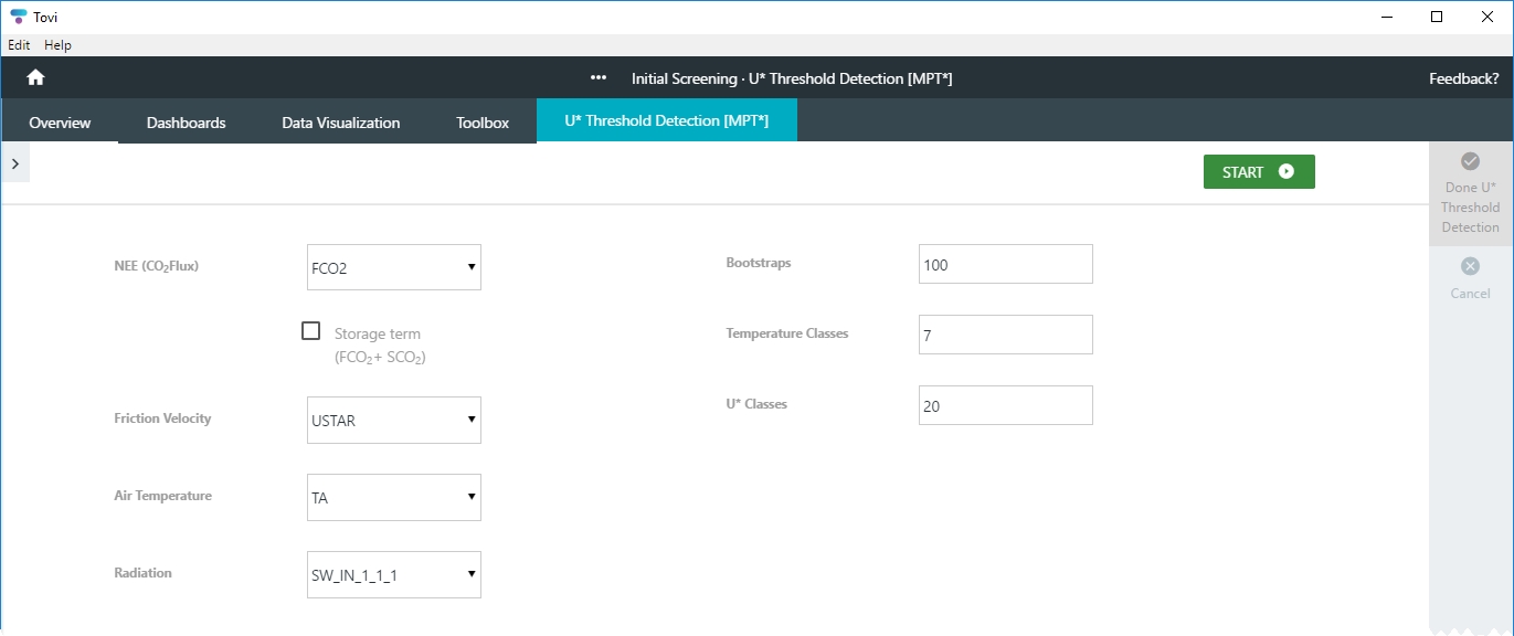
- Click Start.
- Tovi will process data for a few minutes and then present you with results. If using MPT, you'll see one chart for each season covered by your dataset: Winter, Spring, Summer, and Fall (Autumn), and one overall. If using CPD, you'll have a chart for overall results.
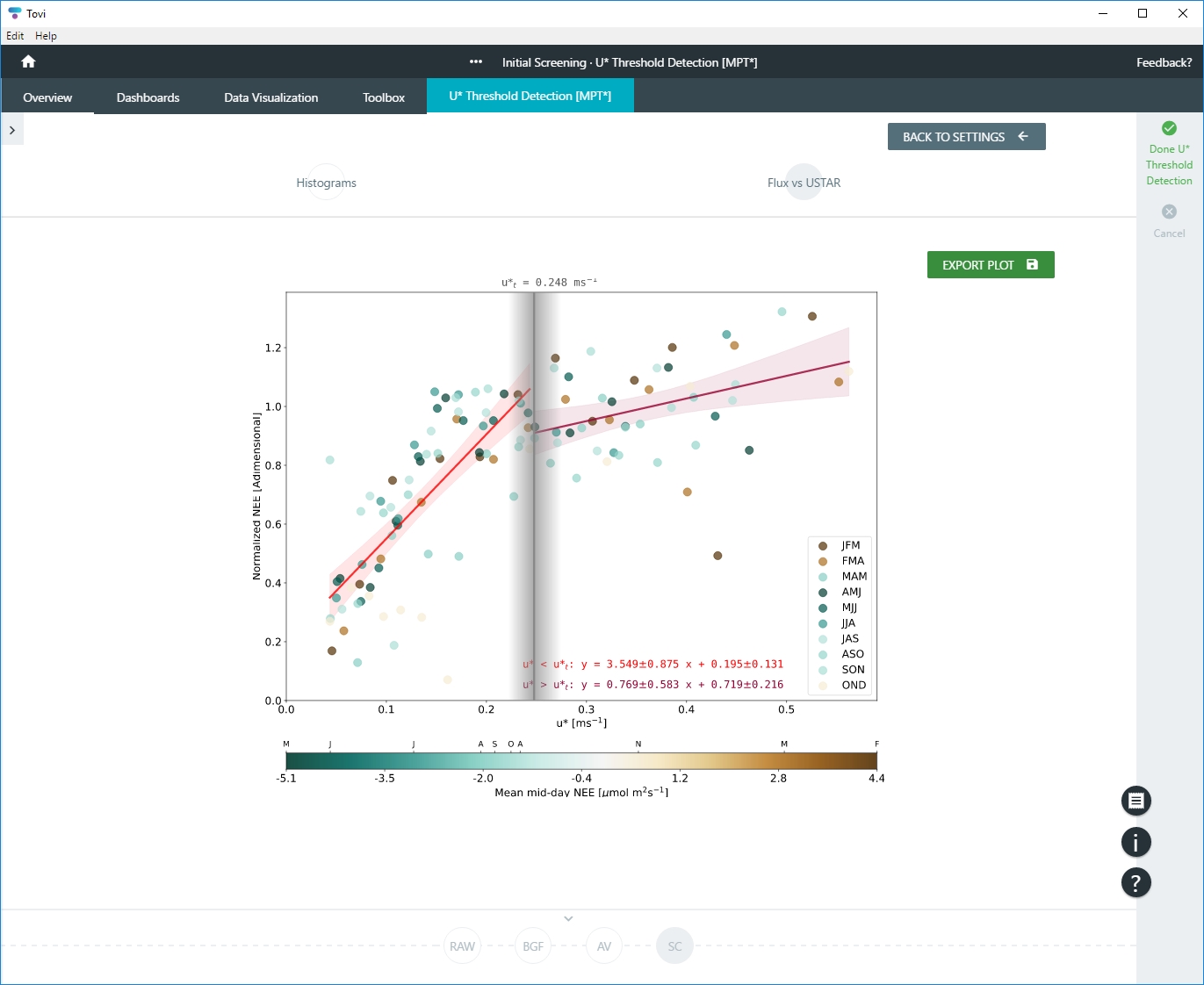
- In addition, you can view the Fluxes vs USTAR, which requires one year of data. For MPT, you'll see a chart with two slopes. For CPD, the chart will have one or more clusters of points. If your CPD plot is poor, consider doing additional QC screening of the data.
- You can save the chart to your computer as an image.
- If you are satisfied with the results, click Done u* Threshold Detection.
- Name the exercise. Tovi will save the information and add a USTAR node to the processing sequence.