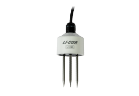
Custom calibrations for the LI-350
The LI-350 is calibrated at the factory to read accurately in mineral soil and soil-less media (such as coconut coir, peat, or potting soil). You can improve the accuracy of the sensor by developing a calibration curve that describes the sensor response in soils with a different composition. Below we provide the steps for a user calibration for the LI-350.
Equipment
The user calibration requires some equipment. Gather everything before you start.
-
Trowel or shovel to collect a bulk sample of soil.
-
Container for samples (e.g., large resealable plastic bags).
-
2-mm sieve to break up clumps.
-
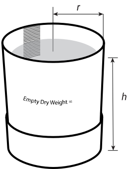
Calibration container with volume sufficient to surround the soil moisture sensor and the volume-of-influence around the probe with sampled soil. A piece of PVC pipe with diameter >20 cm (8 inches) and height >26 cm (10 inches) and an end cap is a suitable container. Weigh the clean, dry container and record the clean dry weight.
-
Drying oven with suitable drying pans.
-
Large scale (capacity >10 kg; resolution better than 0.1 g).
-
Small scale (resolution better than 0.01 g).
-
Soil moisture sensors to be calibrated.
Tips for success
If it is your first time, acquaint yourself with the entire process before you start. Allow several days to complete the full protocol. The adage applies: Plan your work; work your plan.
-
Measure samples promptly after collection. Samples may change in storage.
-
If samples must be stored, keep them closed in a refrigerator or on ice in a cooler.
Custom calibration procedure
The multi-point custom calibration procedure can provide more accurate measurements in situations where soils are dramatically different from the default soil types provided with the probe. You can apply the custom calibration to each sensor to record calibrated measurements, or you can record raw counts from the LI-350 and apply the custom calibration later on a datalogger or with a spreadsheet.
Regardless of when you apply the custom calibration, you'll use the following procedure to develop new coefficients. The steps for applying the coefficients to a custom calibration (C1 or C2) in the sensor are in Applying a custom calibration. The steps for post-processing to convert raw counts are in Converting calibrated counts with a custom calibration. A detailed procedure for custom calibrations follows:
-
Collect a bulk sample of at least four liters of soil.
Samples must represent the soil that will be measured and should be taken from the same depth and general area where the probe will be deployed.
-
Sieve and air dry the soil bulk sample.
Press the soil through a 2-mm sieve to break up clumps and separate rocks and other large particles. Allow the soil to dry in ambient air. Spread the bulk sample in a thin layer in a well-ventilated space to speed up the drying.
-
Determine the mass and volume of the bulk sample.
-
Put the bulk sample into a container and pack it to the same density as in the field.
You may need to add the soil in layers, packing each layer before adding the next. Add or remove soil and record the height in the container (h).
-
Record the mass of the bulk sample (Mbs).
You can either weigh the container with soil and then subtract the container tare weight from the combined weight, or you can place the empty dry container on the balance and tare the balance before adding the bulk sample.
-
Compute initial volume of the bulk sample (Vbs₁).
Use Vbs₁ = π × r2 × h, where r is the radius of the vessel and h is the height of the soil in the container, then record the volume of the bulk sample.
-
-
Determine the volumetric water content of the air-dried bulk sample.
-
Collect a small sub-sample from the bulk sample.
-
Measure the mass of the sub-sample, air-dried (Mssa) using the small scale with fine resolution.
-
Dry the sub-sample.
Spread the sub-sample in a thin layer on a drying sheet and dry at 60 to 70 °C for 48 hours.
-
When drying is complete, obtain the mass of the sub-sample, oven-dried (Msso):
You can either weigh the sub-sample container with the sub-sample and then subtract the container tare weight from the combined weight, or place the empty dry container on the balance and tare the balance before adding the sub-sample.
-
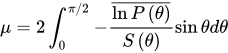
Calculate dry volumetric water content of the air-dried bulk sample (VWCad).
5‑1
-
-
Calculate the dry mass of the bulk sample.
The mass of the bulk sample must be corrected for the initial H2O present:
5‑2
yielding the mass of bulk sample, dry (Mbsd) that will be used for the calibration calculations.
-
Check and set the zero (in air) and full-scale (in water) calibrations (optional).
Although sensors are calibrated at the factory and sensor-to-sensor variation is low, you may improve performance by setting the zero and full-scale readings. Note that this changes the sensor response.
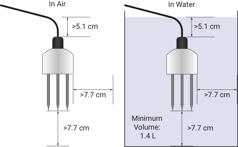
Figure 5‑1. The probe should be far from interfering elements during calibration. While in water, use a volume that is greater than 1.4 L and be sure the tines are at least 7.7 cm (3 inches) from the container walls. -
While the probe is in air, perform the in-air calibration:
Command: aXMA! (use the address of your sensor if different from 0)
Reply: ACK
-
While the probe is in deionized water, perform the in-water calibration:
Command: aXMW!
Reply: ACK
-
-
Record the first calibration data point.
-
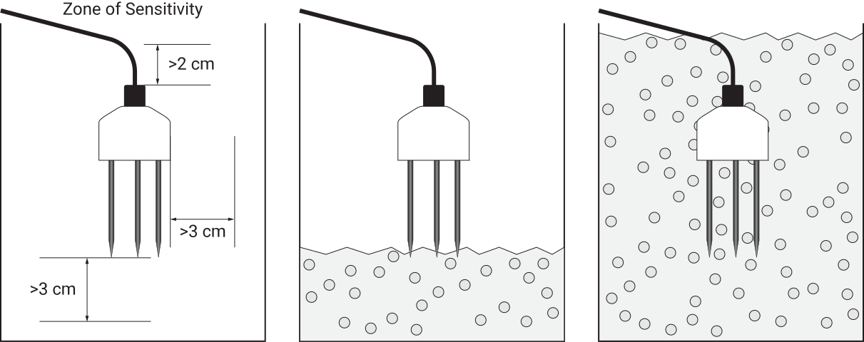
Insert the probe into the bulk sample.
Remove soil, insert the probe, and repack the soil around the probe. For best results, add layers of soil and pack each layer before adding more. Pack the soil to match the bulk density before collection.
-
Record the raw counts reported by each sensor in the air-dried bulk sample.
- Command: aM3! (the measure command).
- Reply: ACK
- Command: aD0! (report measurement group 3).
- Reply: The data (e.g., 0-0.007+0.038+22.96+0+3.05+2928)
The final value in this group is calibrated counts. If using multiple sensors, compute the average of responses at each wetness level. If these values show an appreciable difference from sensor to sensor, that is a clue that there may be a problem with the setup, such as air pockets or voids near tines, for example. Try to determine why you have unexplained variation, then consider redoing the procedure.
-
-
Develop the rest of the coefficients.
With the starting mass of dry media known, the calibration consists of a series of steps where the probes to calibrate are inserted into the soil and a measurement of raw counts made and recorded.
-
Place the bulk sample in a container for mixing.
-
Add a known mass of water.
200 grams of water is a good starting place, but you may need to use more or less. The objective is to assess sensor response to 6 to 8 evenly spaced VWC levels between dry and fully saturated. Choose a mass that accomplishes this.
-
Mix the water with the soil, breaking up clumps and kneading to a uniform consistency.
-
Pack the moistened bulk sample into the calibration container and record the volume, if different from before (Vbs₂).
This new volume is the volume term used to compute VWC at this moisture level. If volume has not changed, use the same value as before.
-
For each addition of water, compute the new mass of H2O and a new VWCg.
5‑3

Mbsw₂ is the mass of the bulk sample after the first wetting. Mbsd is mass of the bulk sample after drying. MH2O₂ is the mass of water in the sample after the first wetting.
5‑4
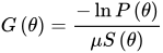
Vbs₂ is the volume of bulk sample after the first wetting. VWCg₂ is the gravimetric volumetric water content (m3 m-3).
-
Install the sensor in the moistened bulk sample.
-
Record the raw counts reported by each sensor for this sample.
-
Repeat these steps until the soil is saturated, creating a calibration curve with 6 to 8 steps.
Table 5‑1. Example of a data table showing sensor response (raw counts) to incremental wetness levels representing cumulative totals. Water
AddedVWCg* Sensor 1 Sensor 2 Sensor 3 Avg. Response None (dry) e.g. 986 e.g. 200 g e.g. 1620 e.g. 400 g e.g., 3585 e.g. 600 g e.g. 4654 e.g. 800 g e.g. 5479 e.g. 1000 g e.g. 7278 e.g. 1200 g e.g. 11225 e.g. 1400 g e.g. 15670 -
-
Generate a calibration function for the soil type using the average sensor response and VWCg*.
You can plot the data in a spreadsheet or with your favorite statistics program. The calibration function will be a fourth-order polynomial, but lower order polynomials may work too. Use your judgment to determine which fits the data best.
The highest-order polynomial leads to VWC = 1 in water. If you are not interested in fully wet conditions and are willing to accept large errors in the full-saturation range, a lower-order polynomial can give better accuracy in a narrower VWC range. This could be useful if, for example, you are interested in high accuracy in the 0 to 50% VWC range, but less concerned with VWC from 50% to 100%.
Furthermore, you can remove unrealistic data points (installation void, poor mixing, data collection error, etc.) from the fit and improve the accuracy of readings in a narrower range of VWCs. The resulting calibration is valid only over its fitted range.
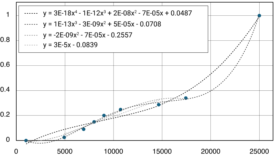
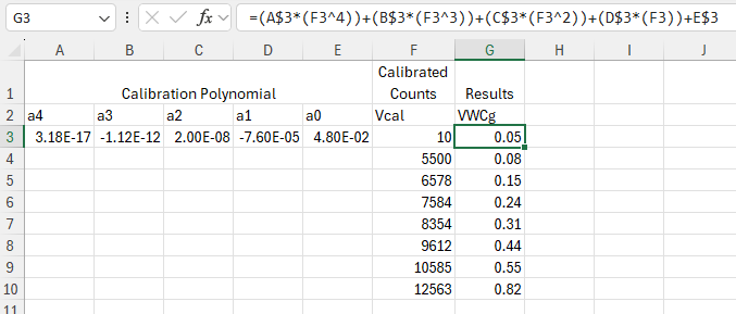
The calibration for a soil type can be determined by a regression of the sensor response and the calculated gravimetric VWC. The coefficients are new values used in equation 7‑2. The LI-350 sensor supports coefficients for up to 4th order polynomial, however a lower order curve may be appropriate, in which case the coefficients for the higher order components can be set to 0.
Applying a custom calibration
After following the procedure to develop custom calibration parameters, you'll load them for one of the custom calibrations (C1 or C2). Be sure you have the coefficients with resolution of eight digits.
Note: Values for VWC coefficients, when displayed as a reply to a user-entered command, are in scientific notation and typically rounded to 5 decimal places. The value you write to them is NOT rounded and is written to memory in “float type” precision. This means the value you write to the sensor is properly being saved but when reported back to you will be rounded.
| Parameter | 4th Order | 3rd Order | 2nd Order | Linear |
|---|---|---|---|---|
| a4 | 3.18259e-17 | 0 | 0 | 0 |
| a3 | -1.12441e-12 | 1e-13 | 0 | 0 |
| a2 | 2.00235e-08 | -3e-9 | -2e-9 | 0 |
| a1 | -7.60457e-05 | 5e-5 | -7e-5 | 3e-5 |
| a0 | 0.048707 | -0.0708 | -0.2557 | -0.0839 |
Here's how:
-
Configure the probe for a custom calibration.
If using a terminal emulator, connect to the probe and use local echo mode so you can see your text entries. Assuming an address of 0, enter the following:
- Command: 0XSTC1! to configure C1 (or C2 for C2)
- Reply: 0Custom1
-
Send the new parameter.
The following command will load the new value for parameter <a4>, using a made up value in place of a4. Use scientific notation for simplicity and eight digits for accuracy.
- Command: 0XVA2.23259E-17!
- Reply: The new value.
-
Check the new value (optional).
- Command: 0XVA!
- Reply: The value for <new parameter>.
-
Repeat this with the other parameters.
Send the commands 0XVB<a3>!, 0XVC<a2>!, 0XVD<a1>!, 0XVE<a0>! with the new parameters. After all new parameters are loaded, the new calibration is available as the custom calibration (C1 or C2).
Note: Values for VWC coefficients, when displayed as a reply to a user-entered command, are in scientific notation and typically rounded to 5 decimal places. The value you write to them is NOT rounded and is written to memory in “float type” precision. This means the value you write to the sensor is properly being saved but when reported back to you will be rounded.
-
Test the calibration (optional).
To confirm the performance of the calibration, it is a good idea to check the zero and full-range readings. For additional assurance, you can check one or more readings with different soil moisture levels.
Converting calibrated counts with a custom calibration
In this example, you'll configure the LI-350 to record calibrated counts. Calibrated counts are normalized to the zero and full range readings. These data are used to apply a custom calibration after the data are logged. You can apply the calibration via a spreadsheet, programmed datalogger, or a computer program.
If you record raw counts instead of calibrated counts, you can apply the calibration to the data, along with the sensor-specific zero and span that normalizes readings from sensor to sensor. You'll use whichever function you choose (three of the four options are likely a poor choice) and the polynomial values in the equation to convert counts to measurements.