Theory and equation summary
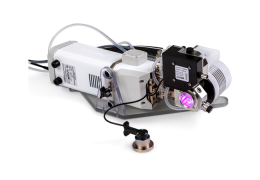
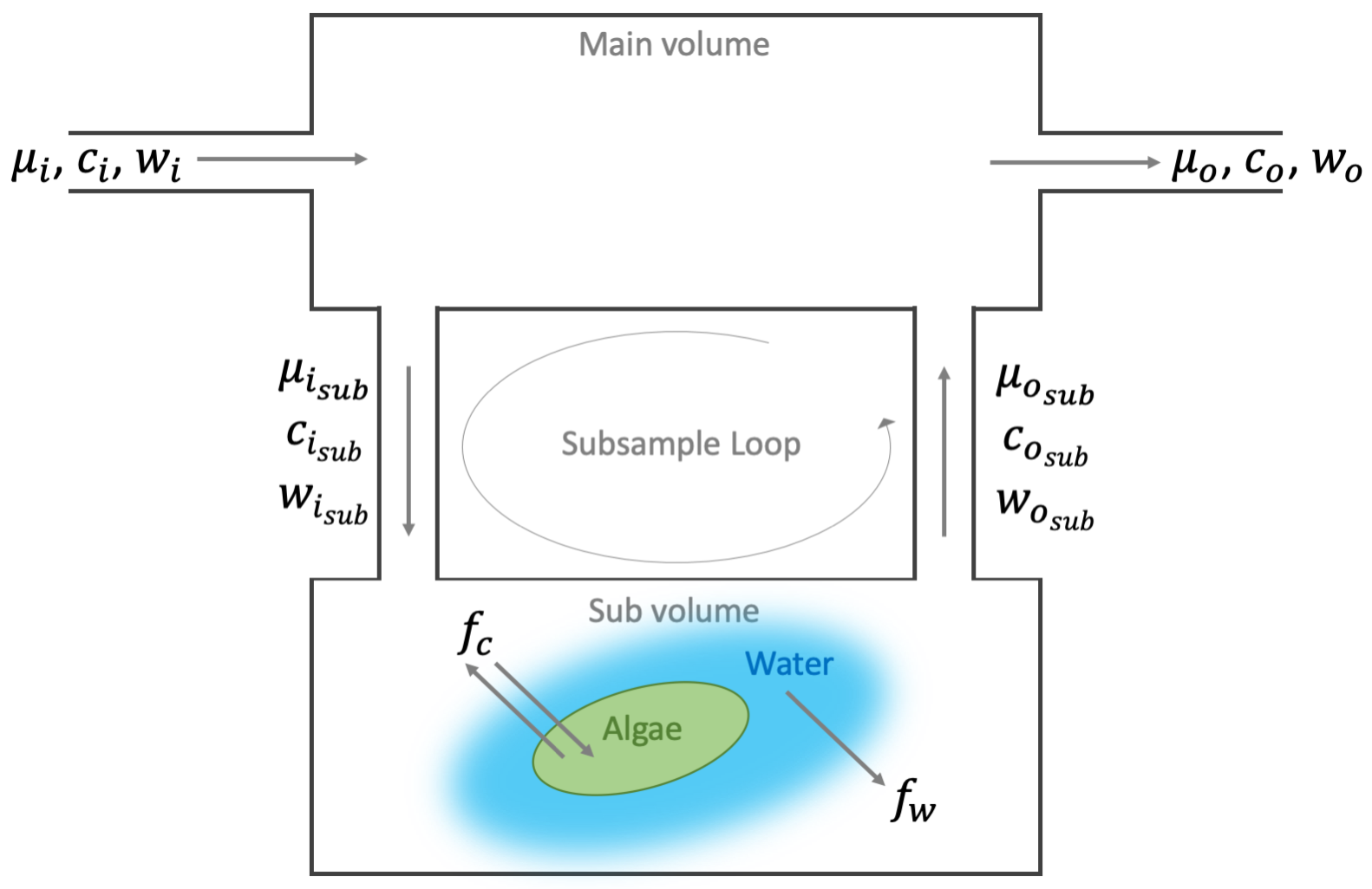
The aquatic chamber is an accessory for the 6800-01A Multiphase Flash Fluorometer on the LI-6800 Portable Photosynthesis System. It replaces the lower half of the fluorometer chamber, allowing chlorophyll fluorescence and carbon dioxide exchange to be measured from a liquid sample (e.g., an algal1 suspension). Figure 10‑1 gives a generalized flow diagram for the chamber.
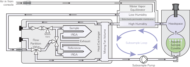
The sample to be measured is held in a cuvette that is in a flow loop parallel to the normal chamber flow path - the subsample loop. Air is drawn from the mixing fan volume into the subsample loop using the subsample pump and returns to that volume after it has interacted with the sample. Air flow into the cuvette is diffused through perforations at the bottom of the cuvette, providing uniform and consistent bubbles for gas exchange between the liquid sample and the air. These bubbles also serve to provide mixing in the liquid sample.
| # | Description |
|---|---|
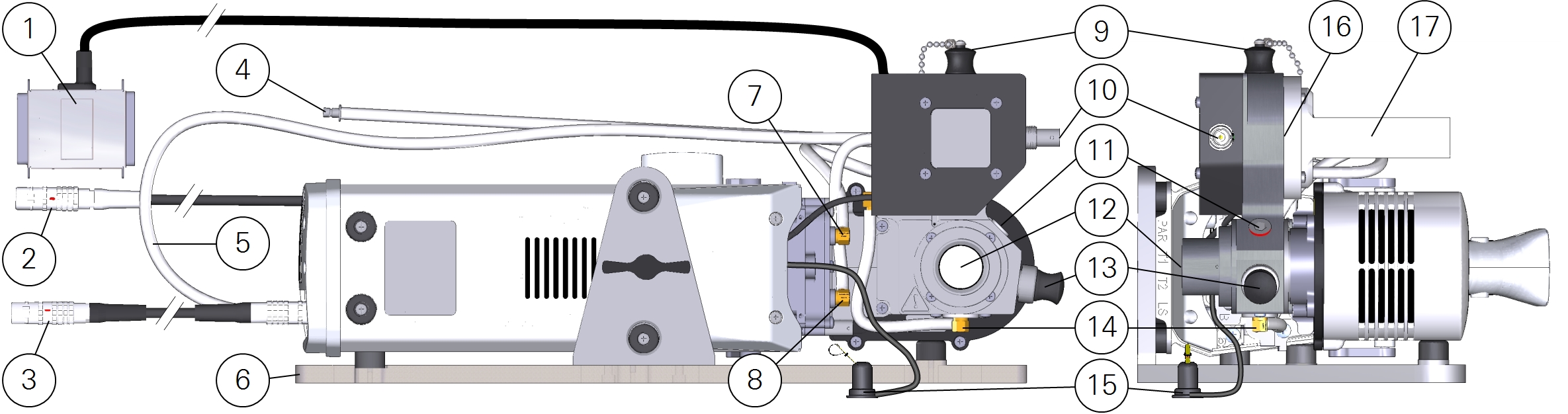
| 1 | Male-to-female DB-25 connector attaches to the USER I/O port on the console |
| 2 | Fluorometer cable connects to HEAD(1) or HEAD(2) on the console |
| 3 | Head cable connects to HEAD(1) or HEAD(2) on the console |
| 4 | Connection for air flow from console |
| 5 | Tube from equilibrator outlet to head inlet |
| 6 | Stand for use with the aquatic chamber |
| 7 | Outlet from mixing volume to subsample pump |
| 8 | Inlet to mixing volume from water vapor equilibrator |
| 9 | Fill port plug. Keep in place during measurements |
| 10 | BNC connector for pH probe analog signal |
| 11 | Silicone PTFE septa |
| 12 | Sample cuvette, quantum sensor port, and observation window |
| 13 | 12-mm diameter O-ring sealed port for a pH electrode |
| 14 | Air inlet to sample cuvette; the inlet PTFE membrane is located here |
| 15 | Ambient air temperature thermocouple |
| 16 | Location of the sample cuvette outlet PTFE membrane |
| 17 | Water vapor equilibrator |
The sample cuvette is isolated on both the air inlet and outlet sides by hydrophobic PTFE membranes. These membranes will only pass liquid water under a significant pressure gradient and thus serve to prevent liquid water from moving from the sample cuvette into the instrument flow path. The subsample pump, however, is strong enough to force water through the outlet membrane. To further guard against liquid entering the air flow path, a set of orientation sensors in the chamber will disable the subsample pump if the chamber is tipped from the normal operating orientation (Figure 10‑2). Overfilling the sample cuvette may also cause liquid water to be forced through the sample cuvette outlet membrane. The recommended working volume for a liquid sample is 15 mL.
After leaving the sample cuvette, air passes through the high side of the water vapor equilibrator before being returned to the mixing fan volume. The total air flow from the LI-6800 console passes through the low side of the water vapor equilibrator before entering the sensor head. Between the low and high sides in the equilibrator is a water vapor selective membrane that allows the exchange of water vapor between the subsample loop and the total system flow. When the total system flow is controlled at an appropriate water vapor concentration, the equilibrator serves two important roles; (1) it brings the near saturated air stream leaving the sample cuvette to a water vapor concentration well below the dew point and (2) it brings the water vapor delta between the reference and sample air streams to a near zero value. This prevents condensation in the instrument flow path and reduces uncertainty in the measurements due to matching and the dilution correction, both of which are described in Minimizing the dilution correction. Details on how to choose an appropriate water vapor concentration to control at are described under Controlling water vapor in the aquatic chamber.
A thermistor embedded near the aquatic sample cuvette measures chamber temperature. Ambient air temperature is measured by a thermocouple (normally used to measure leaf temperature in leaf applications) sitting in the air. The temperature sensors connect to the head via the T1 and T2 connectors. Temperature measurements are visible in the interface and recorded with the data (Taq and Tambient in the GasEx data group).
All other data and power connections are made through the auxiliary connector on the side of the LI-6800 console with a male-female DB-25 connector. The male-female connector passes through those auxiliary channels not used by the aquatic chamber (see Table 10‑1) and blocks access to those that are used by the chamber. Ground (GND), analog ground (AGND), the 12 VDC supply and 5 VDC excitation are all feed-through on this connector and are used by the aquatic chamber. Both the 12 VDC supply (Power12) and 5 VDC excitation (Excite5) are used by the aquatic chamber. These are automatically enabled when the aquatic chamber is selected as the aperture for the 6800-01A.
| Function | Channel | Pin | Description |
|---|---|---|---|
| Pump speed | DAC4 | 5 | Control signal for subsample pump. A 1.5 V set output corresponds to a 4 V supply to the pump, and a 5 V output to a 6 V supply. |
| Orientation | IO7 | 13 | Signal for orientation sensor in the aquatic chamber. When high, the subsample pump is disabled. |
| pH input | ADC8 | 16 | Output from pH sensor amplifier circuit. See Using a pH probe for details on scaling the measured output to pH. |
Mass balance in an open system
The LI-6800 is an open flow through steady-state gas exchange system (here after referred to as an open system) conceptually similar to that modeled in Figure 10‑3.
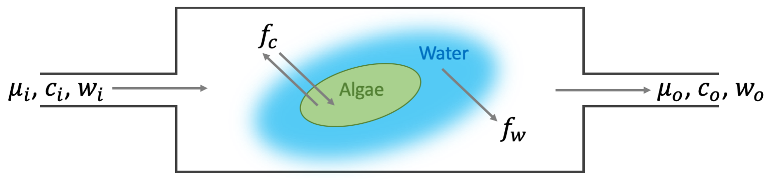
In an open system, a constant flow of gas enters and exits the sample chamber and flux is given by the mass balance between the incoming and outgoing air streams:
10‑1

Where fx is the flux of gas species x (mol s-1), µi and µo are in the incoming and outgoing molar flow rates in mol s-1, respectively, and χi and χo are the incoming and outgoing molar gas concentrations in mol mol-1, respectively2.
The arrangement of the incoming and outgoing terms in the above mass balance changes following the sign convenient for the particular gas species under consideration. Here we consider the flux of two gas species in the context of the aquatic chamber, carbon dioxide (fc) and water vapor (fw), and we use the typical sign conventions for these fluxes following those used in leaf level physiology (a holdover from the LI-6800’s originally intended purpose). fc is positive when carbon is being taken up by the sample and fw is positive when water vapor is lost from the sample. This convention is maintained in the flux calculations used in the aquatic chamber because the implementation of the mass balance used in the LI-6800 to compute fc follows directly from the methodology used for leaf level fluxes.
10‑2

10‑3

Why do we consider the flux of water vapor? In practice, only the flow into the chamber is measured with sufficient accuracy in the LI-6800 to be used in the flux calculation. It is however, not valid to assume that flow in and flow out of the chamber are equal. Indeed, these two flows differ as a function of all gas concentrations that change between the incoming and outgoing flow; i.e., for all gases where flux in the chamber is not zero. Flow out is therefore:
10‑4

For the particular fluxes relevant to the aquatic chamber, and minding their respective sign conventions:
10‑5

Where a particular component flux is small relative to the total flow, that flux is generally ignored when considering its flow effect. For the aquatic chamber, fc is typically 10-5 µi, and its contribution to µo is therefore neglected. fw on the other hand, is closer to 10-1 or 10-2 µi and cannot be ignored. Substituting this definition of µo into the mass balance for fc:
10‑6

10‑7

Noting that fw can be defined independent of itself:
10‑8

Substituting this into the mass balance for carbon dioxide and rearranging gives the form of the mass balance used in the LI-6800:
10‑9

Units of measure in the LI-6800 differ from those expected in the above mass balance. Defining new terms that follow the units of measure implemented on the instrument and substituting into the fundamental mass balance above gives the actual equation used on the instrument. Here incoming and outgoing notation for flows and gas concentrations has been revised to follow the reference and sample notation used in the LI-6800. In the LI-6800, the gas measurements do not follow a serial flow path as might be implied in Figure 10‑3 and the mass balance discussion thus far. Instead, the incoming concentration (now denoted reference) is measured in a parallel gas stream split from the total flow prior to the incoming flow sensor, as shown in Figure 10‑1. The outgoing measurements are denoted sample.
10‑10

10‑11

10‑12

10‑13

Where FC has units of µmol s-1, M has units of µmol s-1, Cx has units of µmol mol-1, and Wx has units of mmol mol-1. FC is reported as the variable Flux in the GasEx data group in the LI-6800. It is the raw flux of carbon dioxide into the sample and has no unit of standardization. In the GasEx group three other fluxes, each with a different unit of standardization are reported. Flux_cell (Fcell) is the flux standardized by cell density (ρcell in cells mL-1), and is reported in µmol cell-1 s-1:
10‑14

Flux_chl (Fchl) is the flux standardized by chlorophyll density (ρchl in µg mL-1), and is reported in µmol µg -1 s-1:
10‑15

Flux_mass (Fmass) is the flux standardized by mass density (ρmass in mg mL-1), and is reported in µmol mg -1 s-1:
10‑16

For all of the above, volume of the sample (V) is in mL.
It is worth noting that the above mass balance discussion implies that the aquatic chamber is a single well mixed volume, which as shown in Figure 10‑1 is not the case. The aquatic chamber is actually composed of two separate volumes connected through a subsampling loop. Under steady-state conditions where there is sufficient flow in the subsample loop and there is no loss or gain between the two volumes (i.e., leaks), this two compartment arrangement has no practical impact on the flux measurement (see Appendix C of the standard LI-6800 user manual for a full derivation of mass balance in a two compartment system; equations C-143 through C-175). This architecture, however, does introduce a concentration difference between the two compartments and this difference may be important under some measurement conditions. Figure 10‑4 provides a model for a two-compartment chamber system similar to the aquatic chamber.
Here we will consider the two compartments as two nested open systems to demonstrate the practical impact on concentration throughout the system. At steady state and in the absence of any leaks between the compartments, the flux in the main and sub compartments must be equal and the mass balance for the two is given by:
10‑17

10‑18

Noting that when the compartment volume is well mixed the outgoing concentrations represent the concentration inside the volume, and since the subsample loop is pulling air directly from the main volume the main volume’s outgoing concentration equals the sub volume’s incoming concentration ( ). Substituting and rearranging to solve for
  :
:
10‑19

Where the flow through the sub compartment is large relative to the magnitude of fw, the effect of including water in the calculation of  approaches zero. For typical measurements in the aquatic chamber, the effect of ignoring water on
  is generally expected to be less than 0.3%. Simplifying to exclude the effects of water yields:
10‑20

For practical purposes, it may be useful to think about the differences in concentration throughout the system in terms of deltas ( in mol mol-1). This is useful in the context of understanding the differences across the two-compartment chamber system, but also because the reported flux is a computed parameter and
  is the fundamental signal being measured to derive that flux. In general, the larger the
  the more confidence we have in the computed fc. The magnitude of
  is controlled by biological activity of the sample, but also by the user set flow rate through the sample chamber, and volume and density of the sample material being measured.
10‑21

10‑22

Following this frame of thinking, the delta between the subsample volume and the main volume ( ) can be defined by the ratio of flow rates between the sample and the subsample flows. This ratio is functionally unitless, and as shown below can be applied without scaling to the deltas:
10‑23

10‑24

The subsample loop flow rate is not measured in the aquatic chamber and is controlled by setting the voltage supplied to the pump in the subsample loop. When the PTFE membranes are clean and there are no additional flow restrictions in the chamber, the flow in the subsample loop scales predictably with control voltage, temperature, and pressure. At the default control voltage (4.5 V), subsample flow rate is approximately 0.38 L M-1. At 25 °C and 101 kPa, that equates to a molar flow rate of approximately 250 µmol mol-1. A method for determining the subsample loop flow rate is given in Measuring the subsample loop flow rate.
As a practical example, when working at the default sample flow rate for the 6800-01A of 600 µmol mol-1, the flow ratio is 2.4. For a  of 10 µmol mol-1, which may be a typical value for a light saturated algal sample at moderate density and 15 mL volume,
  is 24 µmol mol-1 and
  is 34 µmol mol-1 lower than Cr. For a Cr of 400 µmol mol-1, this means the headspace concentration in contact with the sample is 366 µmol mol-1, not 390 µmol mol-1.
The flux of water vapor described previously (fw) represents the flux as relevant for implementing dilution corrections (the term in curly braces in the preceding mass balances), but it should be noted that it does not represent the actual rate of water loss from the sample in the aquatic chamber. The water vapor equilibrator (17 in Figure 10‑2) serves to pass water vapor between the exhaust of subsample loop and the total flow to the sensor head. When properly used, it is adding water from the subsample loop to a partially humidified air stream, meaning that water lost from the liquid sample is contributed to both the sample and reference air streams. To compute the actual rate of water loss from the liquid sample ( ), the total system flow rate (µconsole) and water vapor concentration (wconsole) of the air before reaching the equilibrator must be known:
10‑25

Given the magnitude of the dilution term relative to the carbon dioxide flux under some measurement conditions (e.g., near the light compensation point) it is useful to consider an alternative way of defining the carbon dioxide concentrations. As the flux approaches zero, in the presence of a nonzero difference between Ws and Wr one may well observe the sign of fc is opposite what is expected based on the observed difference in Cr and Cs. This apparent sign reversal is purely a function of the dilution term and is only apparent because Cr and Cs are “wet” values. That is, they are referenced to the actual composition of the air they are measured in and that composition is different with respect to water vapor between the two gas streams.
As is shown by the Ideal Gas Law, at constant temperature (t) and pressure (p), a given volume of gas (v) can only hold a finite number of molecules (n):
10‑26

Where R is the Ideal Gas Constant.
If total number of molecules is comprised of multiple component species ( ), then:
10‑27

And a change in one component will have a resulting impact on all other components. When a diluting gas (nd) is added to the mixture, the sum of the individual components is proportionally reduced
10‑28

10‑29

10‑30

10‑31

where nx is the diluted quantity of the component gas species in the mixture. The term in parentheses above represents the total number of molecules in the mixture excluding the diluting gas. By dividing by n, the above becomes solvable in terms of mole fraction ( ) for a single gas species in the absence of the diluting gas:
10‑32

10‑33

By substituting the water vapor mole fraction for the diluting gas and standardizing to measurement units, this provides a way of referencing the observed carbon dioxide concentrations to dry air, now termed mixing ratio (C'x). Mixing ratios are reported in the Meas2 data group for both the sample (CO2_s_d) and reference (CO2_r_d) air streams and may be useful to monitor in addition to the mole fractions (CO2_s and CO2_r).
10‑34

Note that the mass balance of the mixing ratios is equivalent to the dilution corrected mass balance of the mole fractions:
10‑35

Carbon dioxide equilibrium with water
In following discussion, we will highlight a key assumption linking the biology we are interested in to the measurement we are actually making with the aquatic chamber, and we will provide some framework for understanding and selecting appropriate measurement conditions. Before we do that however, it is important for any user of the aquatic chamber to have some understanding of the behavior of carbon dioxide in equilibrium with an aqueous solution.
For a volume of water in equilibrium with some headspace containing gaseous carbon dioxide ( ), the carbon dioxide dissolved into solution exists in two forms: dissolved gaseous carbon dioxide (
 ) and carbonic acid (H2CO3). Of the two species, the vast majority exists as
  . However, most treatments (including that given here) consider these as a single pool of carbon in solution (i.e.,
  ) and denote that pool as H2CO3.
10‑36

10‑37

The pool of carbonic acid speciates by losing protons to solution. First forming bicarbonate (HCO3-):
10‑38

and from bicarbonate, forming carbonate ( ):
):
10‑39

Under equilibrium conditions, the concentration of carbonic acid in solution ([H2CO3] in mol L-1) is given by Henry’s Law:
10‑40

where K0 is the molar solubility constant and  is the partial pressure of
  , with units of mol L-1 atm and atm respectively.
The equilibrium concentrations of bicarbonate ([HCO3-] in mol L-1) and carbonate ( in mol L-1) in solution are controlled by a set of disassociation constants (K1 and K2) and the pH of the solution (
 ):
):
10‑41

10‑42

The solubility and disassociation constants are controlled by temperature (t in K) and ionic strength of the solution. For an ideal solution, with zero ionic strength, Kx is given by
10‑43

10‑44

10‑45

where ionic strength is non-zero, as in seawater, salinity (S in mg g-1 or ‰) must be considered. Here Kx, now denoted  , is given by:
10‑46

10‑47

10‑48

Note that for practical reasons the solutions given above yield pKx not Kx. pKx is related to Kx by:
10‑49

10‑50

Also note that the above solutions for the disassociation constants represent end points on a spectrum, i.e. freshwater to seawater, which results in some discrepancy in the solutions for Kx and K'x. This discrepancy is controlled by ionic strength of the solution (I), a measure of the salt concentration. For solutions of low salt content, I can be approximated from salinity:
10‑51

The relationships between Kx and K'x, as governed by ionic strength, are given by:
10‑52

10‑53

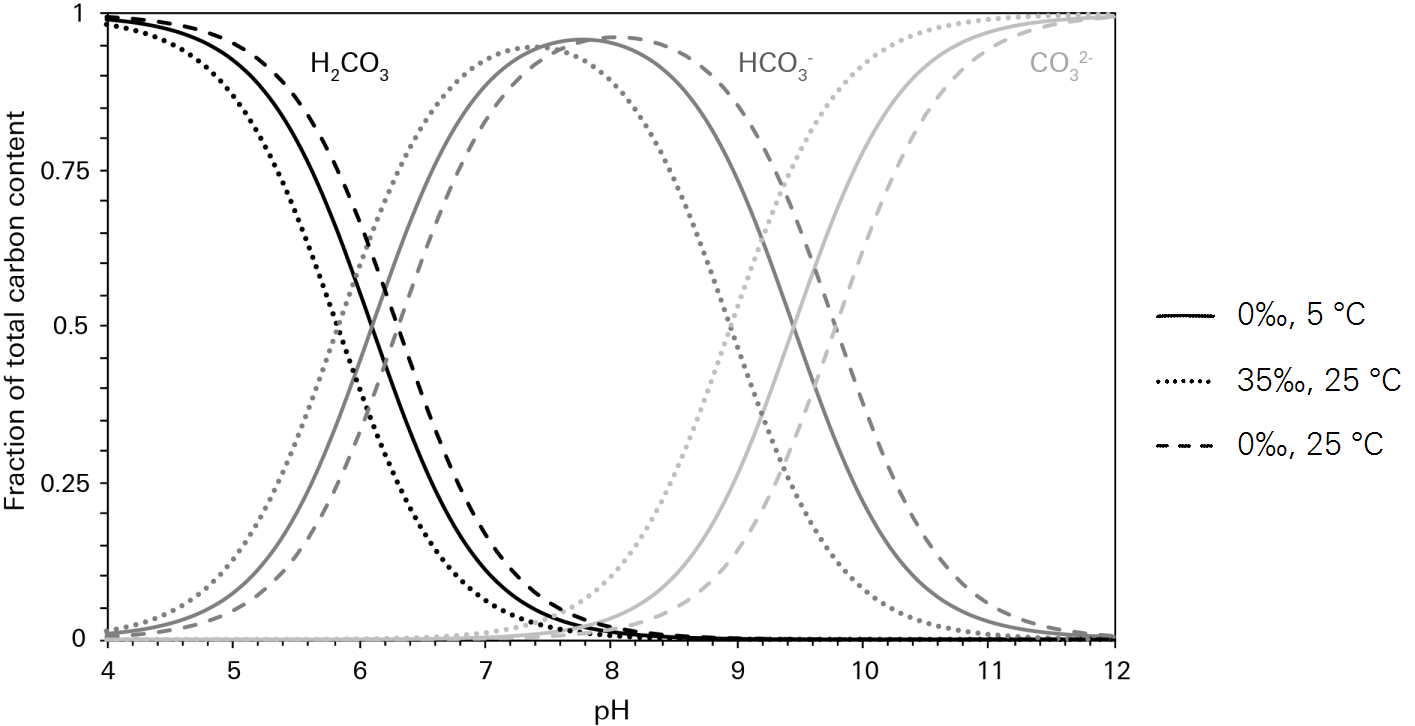
The relationships defined above show that under equilibrium conditions, the total pool of carbon in solution arising from the dissolution of gaseous carbon dioxide (i.e.  ) is controlled primarily by the solubility of carbon dioxide in water, which in turn is controlled by temperature and salinity. How that total pool is then partitioned between the various dissolved carbon species, however, is only weakly influenced by temperature and salinity (Figure 10‑5). The primary driver of partitioning is pH, such that under certain hydrogen ion concentrations the total pool of carbon in solution may be represented almost entirely by a single species.
Carbon dioxide exchange with a liquid sample
The relationships defined in the previous section are useful in the context of understanding the partitioning of various carbon species in solution under equilibrium conditions. Achieving that equilibrium state is controlled not by partitioning however, but by mass transfer at the air/water interface (see Figure 10‑6) in the sample cuvette, and can be described by a modified form of Fick’s Law for the two phases involved:
10‑54

10‑55

where f is the mass transfer, or flux, of the gas species (mol s-1), a is the interacting surface area at the air/water interface (m2),  is the mass transfer coefficient for the particular phase (mol m-2 s-1 atm-1 or m-2 s-1 L, depending on phase), pgas and pinterface are the partial pressures of the gas in atm in the bulk air and at the air/water interface respectively, and cinterface and cliquid are the liquid phase concentrations in mol L-1 of the dissolved gas at the air/water interface and in the bulk solution respectively.
When the gas and liquid phase concentrations are at equilibrium with no net accumulation of the gas species in either the air or liquid phase, the diffusion gradient (the terms in parentheses above) collapse and the flux goes to zero. The time it takes to reach this state will depend on the magnitude of the diffusion gradient, interface surface area, and the magnitude of the two mass transfer coefficients. It’s useful to consider the flux in the context of a total mass transfer coefficient ( ):
):
10‑56

which represents the combined effects of the individual transfer coefficients:
10‑57

It is apparent here that the total mass transfer may be dominated by the mass transfer in one phase or the other and is controlled in part by the solubility of the gas in solution.
When there is a net accumulation of the gas species in one phase or the other (e.g., when a photosynthetically active organism is in the sample cuvette), the flux will be a non-zero value. It is important to note here, that the total measured flux is the flux across the air/water interface. In this case, to measure a total flux which is representative of the rate of accumulation in one phase or the other (e.g., the photosynthetic carbon accumulation rate), it is assumed that the total mass transfer coefficient is sufficiently large as to not be limiting. This assumption is valid where a steady-state flux is observed.
When the flux is not at steady-state, one end point of the diffusion gradient or the other must be changing, as the interface surface area and the mass transfer coefficient are expected to be more or less constant in the aquatic chamber. The change in the diffusion gradient will be driven by a change in the accumulation rate in one phase and/or by movement of dissolved gas in the liquid phase into equilibrium with the sample cuvette head space concentration. As such, the time required to reach a steady state in the sample cuvette will be dependent on how different the solution concentration is from the equilibrium concentration.
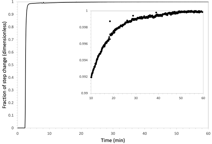
Thus far, the discussion of mass transfer limitations has considered the dissolved gas in solution as a single pool representing a single end point of the diffusion gradient. However, as shown above, carbon dioxide dissolved in solution partitions into a variety of species dependent on the solution pH. As such, it is important to consider the balance of the three primary end point concentrations (for typical measurement conditions anyway) on the final equilibrium state: these are the head space [CO2], pH and [HCO3-]. These three are interdependent on each other and individually manipulable, such that it cannot be assumed that a liquid sample is in an equilibrium state before it enters the sample cuvette. Once in the cuvette, active mixing with the measurement air stream will eventually force an equilibrium. However, the further these three are from equilibrium initially, the longer this will take. Figure 10‑7 shows a time-to-equilibrium example where a 15 mL water sample at 17 ‰ salinity and buffered to a constant pH of 7.0, was taken from equilibrium with a head space [CO2] of 600 µmol mol-1 to equilibrium at 400 µmol mol-1. In this case, the head space concentration change drove carbon dioxide out of solution decreasing the [H2CO3] and subsequently that of [HCO3-] while [H+] remained constant. The total time to reach the new equilibrium was approximately 50 minutes, with the bulk of that time being dominated by the last 1% of the step change. It should be noted that the observed carbon flux during the last 1% of the step change was on the order of magnitude of typical carbon fluxes observed in the aquatic chamber for algal suspension.
Under some algal cultural conditions, the growth media may be supplemented directly with a bicarbonate source, with or without addition of a separate pH buffer. Where mass transfer between the atmosphere and the algal culture is sufficiently low (as is often the case with lab grown cultures) the carbonate system may not be in equilibrium with the atmosphere, and that additional bicarbonate will stay in solution where it remains available as a substrate for photochemistry. In the aquatic chamber however, where mass transfer between the head space and liquid sample is favorable, the liquid sample will be forced to equilibrium and the bicarbonate in solution will be lost as carbon dioxide to the cuvette headspace. The further from equilibrium conditions between the sample and the head space [CO2] initially, the longer it will take to reach equilibrium, and thus a steady state in the sample cuvette.
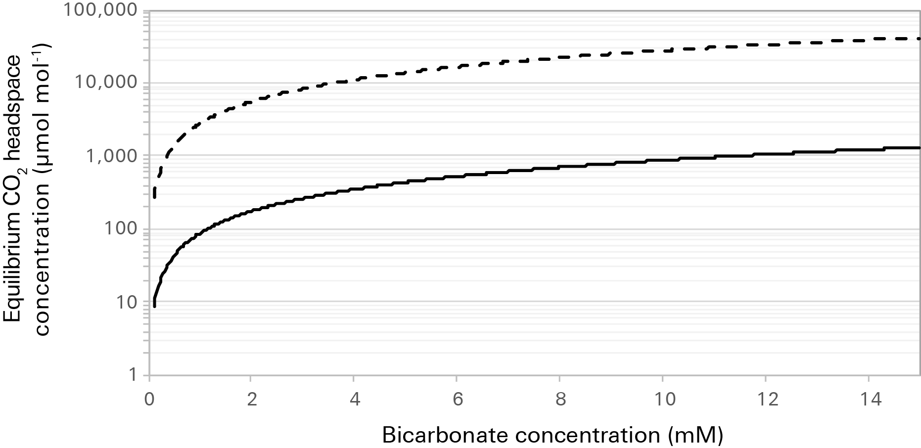
Figure 10‑8 gives equilibrium head space concentrations of carbon dioxide for a range of bicarbonate concentrations at 25 °C and two pH values. Where bicarbonate is supplemented directly in the culture media, it may be more useful to consider the equilibrium [CO2] as opposed to the atmospheric [CO2] when choosing a [CO2] to make measurements at. At the same time, it is important to be mindful of pH. Where pH is low and [HCO3-] is high, the equilibrium [CO2] may quickly exceed the measurement (3100 µmol mol-1) and control (2000 µmol mol-1) ranges for carbon dioxide by the LI-6800.
Achieving steady-state conditions
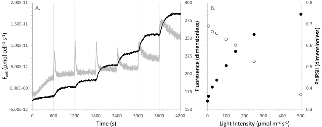
The time required to reach to a steady state can be reduced in the aquatic chamber by the addition of carbonic anhydrase to the sample media. Carbonic anhydrase facilitates the interconversion between CO2 in solution and bicarbonate, increasing the rate of this interconversion over the rate at which it happens naturally. Any addition of carbonic anhydrase can be expected to provide some improvement in how quickly steady state is reached. Excess carbonic anhydrase is not expected to negatively impact measurements. For typical measurements, anything greater than 0.5 mg of carbonic anhydrase added to a 15 mL sample provides sufficient reduction in the time to steady state. Figure 10‑9 gives an example of time-to-steady state during a measurement of the carbon assimilation response to light intensity in a Chlorella sp. suspension (i.e., a photosynthesis irradiance curve). Data were collected in an F/2 growth media at half seawater salinity with no additional pH buffer and 0.5 mg of carbonic anhydrase added to the solution. Here, the time it takes the carbon flux to reach steady state is relatively constant when moving between light intensities and tends to lag just behind the steady state fluorescence, indicating that much of the equilibration time at each light intensity is driven primarily by biology.
In several of the example data sets, pH was held constant with a buffer that acts independent of the carbonate system and the [CO2] entering the chamber was held constant (CO2 reference control). Where pH is not independently buffered in the measurement solution, it should be noted that changing the head space concentration or the accumulation rate in the liquid phase, will result in a concurrent change in the pH of the sample. In a series of light response measurements on an algal suspension using reference CO2 control for example, the net effect of this would be a steadily increasing pH as the sample is further illuminated. Whether this change in pH is large enough to be important will depend on how large the change in solution CO2 concentration is during the measurement series, which in turn will be a function of algal density, photosynthetic rate, and the ratio of sample to subsample flow rates. In the absence of an appropriate buffer, this pH effect may be partially ameliorated by using sample CO2 control to keep the mixing fan volume concentration constant through the measurement series. The tradeoff being that for measurements of small signals (of low photosynthetic rate and/or low algal densities), feedback in the CO2 control may be more apparent as noise in the carbon flux measurement, necessitating increased averaging times and longer time to steady state. For the photosynthetic rates and sample densities encountered during development of the aquatic chamber, the change in head space [CO2] observed across typical light response measurement was on the order of ~30 µmol mol-1, which roughly corresponds to a change of a little over 0.2 pH in a completely unbuffered sample.
Three general recommendations can be derived from the above:
- Measurements made on a liquid sample that is already at equilibrium with the measurement conditions will be significantly faster than when the sample much reach equilibrium in the cuvette. The best practice is to re-suspend the sample cells in fresh pre-equilibrated media prior to placing them in the cuvette for measurements.
- Where measurement conditions will be very different than cultural conditions with respect to CO2 concentration, or where large changes in CO2 concentration are expected during the measurements, pH in the measurement solution should be buffered with an appropriate buffer that acts independent of the carbonate system.
- The addition of carbonic anhydrase to the sample will improve time-to-steady state and is recommended as a best practice for measurements in the aquatic chamber.
Controlling water vapor in the aquatic chamber
As described previously, air leaving the sample cuvette of the aquatic chamber passes through an equilibrator that allows for exchange of water vapor between the sample cuvette out flow and the total flow to the sensor head. The equilibrator is intended to serve two key functions in the aquatic chamber: (1) to bring the outlet air stream from the sample cuvette to a water vapor concentration well below dew point and (2) to minimize the difference in the water vapor concentration between the reference and sample air streams (Δw = Ws - Wr).
Avoiding condensation
To achieve the first, the air passing through the low side must be sufficiently less than saturated at the ambient temperature outside the chamber. The equilibrator and flow return to the mixing fan volume are both exposed to the ambient environment. Depending on air movement around the chamber, these will be somewhere near to a little above the ambient temperature. Controlling water vapor at a concentration near saturation will generally result in condensation forming in the chamber air return and collecting in the mixing fan volume.
Caution: Excessive water accumulation in the mixing fan may cause immediate damage to the match valve or the sample gas analyzer. Water left in the mixing fan volume will damage the instrument over time.
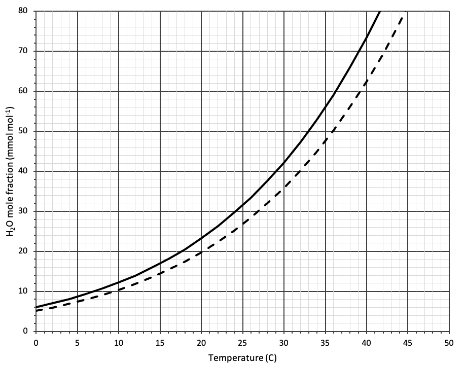
To ensure that air returning from the chamber to the mixing fan volume does not form condensation in the instrument, control on a water vapor mole fraction in the reference analyzer that ensures the sample air stream is not saturated at the ambient temperature. Figure 10‑11 shows the saturation water vapor mole fraction (solid line) as a function of temperature at 101 kPa atmospheric pressure. Note that as pressure decreases, the saturation mole fraction increases linearly: at 50.5 kPa it is two times the mole fraction at 101 kPa (see Useful water vapor calculations). In practice, basing the control choice on saturation mole fraction is risky. Small temperature gradients in the system may mean that parts of the flow path are cooler than the nominal ambient value, and as such we recommend controlling below the saturation mole fraction at 85% relative humidity. This is the default threshold used for condensation warnings in the LI-6800. For example, for measurements made in a 22 °C room and where 1 mmol mol-1 Δw is achieved, controlling at a reference mole fraction of 20 mmol mol-1 should ensure condensation-free operation.
The LI-6800 is capable of automatically guarding against condensing conditions in the system. By default, it will use the lowest measured temperature to trigger warnings and water vapor control lock outs to prevent condensation. The instrument does not have a built-in ambient air temperature measurement however. For users who wish to take advantage of this functionality to prevent condensation in the exposed portions of the aquatic chamber flow path, connect the leaf temperature thermocouple (from the standard chamber bottom of the 6800-01A fluorometer) to the open temperature input on the bottom of the sensor head and leave the thermocouple in a location representative of ambient temperature. The LI-6800 will automatically consider this temperature when evaluating the risk of condensation.
In general, the concentration gradient will typically favor the movement of water vapor from the high side (chamber side) of the equilibrator to the low side (console flow side). However, the rate of water vapor transport is limited by the membrane surface area, temperature of the equilibrator, and the difference in water vapor concentration across the membrane in the equilibrator, such that for most water vapor concentrations on the low side of the equilibrator some difference between the water vapor concentrations in the reference and sample air streams is maintained. Figure 10‑10 shows the relationship between Δw and the water vapor concentration measured in the reference air stream.
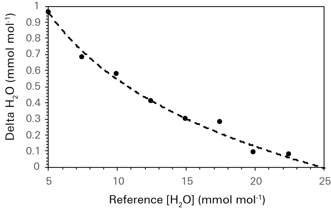
This data set was collected at a nominal room temperature of 22 °C, a liquid sample temperature of 20 °C, and a subsample pump supply voltage of 5 V. Under the measurement conditions, 5 mmol mol-1 of water vapor in the reference air stream was about the lower limit of water vapor control by the LI-6800. This represented full air flow through the desiccant and is significantly greater than the expected 0 mmol mol-1 in the reference air stream because of the contribution of water vapor form the sample cuvette out flow to the reference airstream through the equilibrator. Controlling the water vapor concentration in the reference analyzer at 5 mmol mol-1 yielded a Δw between the sample and reference air streams of approximately 1 mmol mol-1, which is in the range of typical Δw values for leaf level measurements.
Minimizing the dilution correction
The smaller the Δw, the less uncertainty is introduced to the carbon flux measurement by the water vapor measurement. The delta matters considerably more here than the absolute value of the water vapor concentration for these measurements. Where a large delta exists, matching the IRGAs with an air stream at a water vapor concentration different than the measurement water vapor concentration introduces uncertainty in the match correction due to the nonlinearity of the analyzers and through inherent cross sensitivities between the carbon dioxide and water vapor measurements.
Water vapor appears additionally in the carbon dioxide flux equation in the form of a dilution correction (see Mass balance in an open system above). The magnitude of this dilution correction scales proportionally with Δw, and where Δw is not actively minimized, the magnitude of the correction easily exceeds the magnitude of the flux it is applied to when working with samples in the aquatic chamber.
The response of the equilibrator to a change in water vapor concentration is not instantaneous. It takes on the order of minutes to reach steady state after the water vapor concentration is changed. Noting this will be important in the context of starting measurements, particularly if the chamber has been unused for a long period of time, and when a change is made to the reference water vapor concentration setpoint.
Useful water vapor calculations
The saturation vapor pressure for moist air ( in kPa) at a given temperature:
10‑58

Where β is a dimensionless enhancement factor accounting for temperature and pressure effects. For temperatures between 0 and 50 °C and pressures above 80 kPa, assuming a constant value of 1.004 for β contributes negligible error to the computed vapor pressure. Outside that range β can be computed as:
10‑59

Where P is atmospheric pressure in kPa.
The water vapor mole fraction can be computed for a given relative humidity (RH, in %) from saturation vapor pressure:
10‑60

Pulse-Amplitude Modulation fluorometry
The LI-6800 employs two techniques to evaluate chlorophyll a fluorescence: measurements of fluorescence emission with a pulse-amplitude modulation (PAM) fluorometer, and measurements of maximum fluorescence yield upon application of a saturating flash of light. These are described in detail for both leaf and aquatic applications in Fluorometer theory and equation summary. Considerations for aquatic samples are described in Chlorophyll a fluorescence in algae suspensions.
Chlorophyll a fluorescence in algae suspensions
The 6800-01A fluorometer was originally developed for use with optically dense samples of tissue from higher plants, specifically leaves. When using the 6800-01A with optically dilute samples, such as algal suspensions, certain aspects of how the instrument detects fluorescence need to be paid particular attention. Figure 10‑12 shows relative fluorescence emission spectra as measured by an LI-1800 spectroradiometer for a soybean leaf and a Nannochloris suspension, both normalized to their respective relative emission at 700 nm. In the Nannochloris suspension, peak emission happens at about 685 nm and fluorescence emission above 700 nm is greatly reduced relative to that at wavelengths below 700 nm. In the optically dense soybean leaf, peak emission happens well above 700 nm with relatively little of the total emission occurring below 700 nm. The difference in peak fluorescence emission between these two samples is related to the abundance and spacing of the photosynthetic pigments. In optically dense materials, where the photosynthetic pigments are abundant and tightly grouped together, the opportunity for absorption of fluoresced photons at photosynthetically usable wavelengths is high. As such, the fluorescence escaping the sample at wavelengths below 700 nm is greatly reduced compared to that above 700 nm. In optically dilute samples, the density of the photosynthetic pigments is lower. Increased spacing between pigments reduces the opportunity for absorption of fluoresced photons at the photosynthetically usable wavelengths and shifts the relative emission preferentially toward lower wavelengths.

In the context of the 6800-01A the spectral shift in fluorescence emission with optical density is important. The 6800-01A fluorescence detector is long-pass filtered with a nominal cutoff wavelength of 700 nm, such that it is relatively blind to fluorescence emission below that wavelength. This detection scheme does not invalidate the 6800-01A for use with algal suspensions (or any other optically dilute sample material), but it does mean that the raw fluorescence detected by the instrument will be lower than if working with an optically dense sample in a comparable physiological state. Figure 10‑13 shows a time series of fluorescence as reported by the 6800-01A for a suspension of the golden algae Isochrysis galbana, with peak emission of about 205 fluorescence units at the highest modulation frequency. In comparison, typical fluorescence emission from a healthy leaf measured in the same manner shows values on the order of three to six times this.
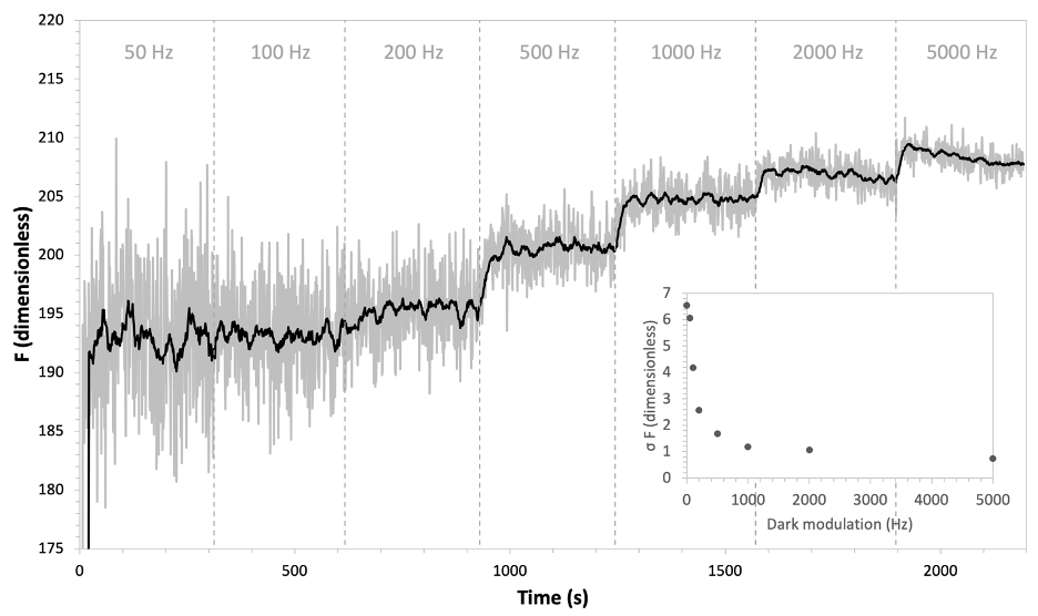
With this lower signal, optimizing dark modulation frequency becomes quite important. With increasing dark modulation frequency, the number of samples included in the averaged fluorescence signal increases. The positive effect of which, as shown in Figure 10‑13, is that noise in the signal is decreased such that at a higher modulation frequency the signal-to-noise ratio becomes more favorable. However, there is a potentially negative effect: at higher modulation frequencies the possibility of inducing photochemical quenching becomes more likely (i.e. violating the assumption of  ). In Figure 10‑13, the fluorescence emission increases when the modulation rate is increased past 100 Hz. The rise in fluorescence with each subsequent rise in modulation rate suggests that any modulation frequency above 100 Hz is likely too high to be used for measurements because it may be invalidating the underlying assumption of physiological state required for measurement of minimal fluorescence in the dark (Fo).
Increasing the averaging window used for determination of fluorescence parameters on the instrument may also be considered for improving the signal to noise ratio. The default averaging window is 15 seconds and can be changed under user control. Do note that the averaging window determines the minimum amount of time the sample must be in the chamber and at a physiological steady state before a flash can be given, and as noted below may be an important constraint to consider in algae specific measurement protocols of Fv/Fm.
Rectangular or multiphase flash?
The 6800-01A supports two protocols for providing saturating flashes during a fluorescence measurement: a rectangular flash protocol where light intensity is raised and held at a constant value for some period of time (as described in Pulse-Amplitude Modulation fluorometry) and a multiphase flash protocol where the light intensity is varied during the flash. To date, no work has been done validating the use of the multiphase flash protocol in the 6800-01A on algal suspensions and as such no recommendations for its use are reported here. All existing work has been done using the rectangular flash protocol.
Physiological considerations
Algae can exhibit some unique physiological behavior that may impact fluorescence emission during the flash and in turn have an impact on final reported values of fluorescence parameters. It is important to note that some of these behaviors need to be considered in the context of the measurement configuration and some simply mean that reported fluorescence parameters, even when measured correctly, will be markedly different than what are generally accepted as expected values (note that most “expected values” come from measurements on higher plants). The maximum quantum efficiency, Fv/Fm, for example, measured on healthy algal cultures will typically be below 0.8, and its maximum will vary depending on the pigment composition of the particular taxonomic group of the algal species being measured. However, despite the expected lower values of Fv/Fm when measured correctly, Fv/Fm may be further reduced in measurements of algal suspensions by physiological processes that invalidate the underlying assumptions of the measurement.
State transitions
The variable fluorescence signal that is detected during a fluorescence measurement as done by the 6800-01A, is primarily controlled by the states of the PSII reaction centers and associated downstream components of the photosynthetic machinery. This fluorescence arises from light energy captured by the light harvesting complexes, particularly LHCII, in the antenna array associated with PSII and is intrinsically linked to the capacity for energy transfer between LHCII and PSII. In higher plants, LHCII is predominately locked to PSII, such that under most conditions the bulk of energy captured by LHC II is funneled to the PSII reaction center. In many algal species however, the connection between LHCII and PSII is plastic such that energy transfer from LHCII to PSII is not always favored. LHCII is migratory in these systems and can become preferentially connected to PSI, at which point, the bulk of the energy captured by LHCII is funneled directly to PSI, not PSII. The transition in association of LHCII between PSII and PSI is commonly referred to as a state transition, where state I represents the LHCII-PSII association and state II the LHCII-PSI association, with an intermediate state existing as LHCII transitions between associations. If a larger proportion of LHCII complexes are in state II, variable fluorescence is reduced as the role of PSI in quenching captured energy increases and less energy is transferred to the PSII reaction center. A consequence is that maximum fluorescence in the dark, Fm, is reduced relative to Fm measured with a larger proportion in state I. The impact of state transitions only changes Fm, with Fo remaining unaffected. The net result of which is that dark-adapted parameters, such as Fv/Fm, will be underestimated in cases with a large proportion of state II.
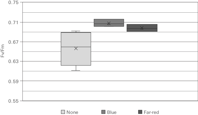
State transitions occur on the time scales of seconds to minutes in algae, and likely are important in optimizing energy partitioning between the photosystems as light intensity changes. For algae in the dark or under dim light, state II may be favored. In this case, accurate estimation of Fm requires transition to state I before a fluorescence measurement is performed. Transition to state I is generally achieved by exposing the sample to a low intensity of light preferentially absorbed by PSI (typically in the blue or far-red region of the spectrum). In the aquatic chamber this can be done using the blue or far-red LEDs in the 6800-01A fluorometer and should be routinely evaluated when developing a protocol for measuring Fv/Fm. This pre-treatment prior to the dark-adapted measurement may also be useful in opening up the plastoquinone pool in the presence of chlororespiration, resulting in a reduction in Fo. The need for pre-treatment may change with cultural conditions, growth stage and stress, and will vary between species.
Figure 10‑14 shows the effect of pre-treatment light on Fv/Fm measured on a Chlorella species. The data clearly shows an enhancement in Fv/Fm after exposure to a weak light preferentially absorbed by PSI. The somewhat stronger effect after blue versus far-red exposure may suggest that both chlororespiration as well as state transitions are active in this sample.
Averaging time and response time considerations
When a blue light pre-treatment is used prior to dark-adapted measurements, it should be noted that the recovery times associated with the state transition and chlororespiration effects will likely be much quicker than that of the measured carbon flux. This difference in time response means that the measurement of dark respiration and the dark-adapted fluorescence with a blue pre-treatment must be decoupled. In this case it is recommended to measure the dark respiration rate first, followed by a suitable blue pre-treatment/flash series. If a saturating flash is given during the initial dark respiration measurement, a suitable delay should be included between this flash and the post pre-treatment flash to allow re-acclimation to a dark-adapted state. Additionally, it is important to be mindful of averaging times when developing a pre-treatment protocol. For Fo a 15 second averaging window is applied by default, meaning that for a flash given less than 15 seconds after the pre-treatment light is turned off, Fo will include data from when the light was on. When far-red light is used for pre-treatment this is particularly problematic as the far-red light is visible to the fluorescence detector used in the 6800-01A.
For a well configured saturating flash, dark-adapted algal suspensions may not exhibit fluorescence emission that closely follows the rectangular nature of the flash as would generally be expected. Rather, the fluorescence emission during the flash may exhibit multiple distinct phases each representing different physiological mechanisms. Figure 10‑15 shows fluorescence emission during a rectangular flash done with a dark-adapted suspension of photo-autotrophically grown Chlorella. Upon illumination during the flash, fluorescence begins to rise towards a maximum emission, reached at about 200 ms in this dataset. This initial rise is biphasic in nature and represents the contributions of a thermal and a photochemical phase to the induction of fluorescence quenching. Following the observed maximum fluorescence, there is a marked decline in the fluorescence emission that is likely the result of quenching due to oxygen dependent electron flow. The shape of the fluorescence emission shown in Figure 10‑15 is predominately independent of the flash intensity, meaning that increasing or decreasing the flash intensity does not eliminate the biphasic nature of the rise nor does it suppress the post maximum decline. The degree to which a given algal suspension exhibits the behavior shown in Figure 10‑15 will likely be influenced by species and culture conditions. Particularly, dark-adapted measurements on heterotrophically cultured algal suspensions, where the partial pressure of oxygen in solution may be quite low, may not show the post maximum decline.
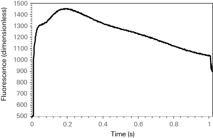
Rectangular flashes on algal suspensions are typically kept quite short, such that little of the post maximum decline (if present) is included in the measurement. The way that maximum fluorescence is derived in the 6800-01A makes the determination of Fm independent of any inclusion of the post maximum decline during the flash. However, short flash durations are still recommended as best practice for dark-adapted measurements on algae in the 6800-01A. Flash duration should be long enough for fluorescence to reach a maximum following the initial biphasic rise and short enough not to include the post maximum decline. For the species and culture conditions encountered during development of the aquatic chamber, flash durations of 250 to 500 ms were typically sufficient. This however, should be evaluated by the user for their particular sample material.
Additionally, it is worth noting that many algal groups contain a variety of secondary pigments which may or may not influence fluorescence at the wavelengths detected by the 6800-01A fluorometer. Fluorescence from these secondary pigments may invalidate the assumptions of the measured fluorescence parameters. Some phycobilins, such as phycocyanin found in Cyanophyta, contribute to non-variable fluorescence above 700 nm. The result is an increased Fo and subsequent reduction in values of Fv/Fm. This obviously invalidates the normal assumption that Fv/Fm, as measured by 6800-01A, is representative of the quantum efficiency of PSII since it contains artifacts from phycocyanin in these organisms.