Custom flash events
Custom flashes allow you to define up to 38 steps to be executed during a flash, and in each step specify duration, modulation rate, output rate, red intensity, blue intensity, far red intensity, modulation beam peak intensity, and rate of change of red actinic intensity. We’ve used the term “flash”, but more generally this is an event, since it could be a dark pulse, or flash and a dark pulse, or any combination of things you’d care to define.
There are two parts of a Custom event definition:
-
What happens during the event.
This is determined by a series of steps that specify settings and durations. These steps can be viewed or edited in a table (The table editor).
-
The results and computations that are to be extracted from the event data.
This is controlled by a list of commands that you specify (Meta commands).
Custom flashes are configured from the Fluorometry > Settings > Custom screen. A tour, with an example of how to use this screen, follows next.
A quick tour
For this tour, we begin by examining a custom flash that performs a multiphase flash. Then, we'll add some steps at the start to measure the initial rise (OJ) under a very brief saturating pulse prior to those doing the those MPF steps.
-
In the Settings > Custom screen, tap New, pick Multiphase, and tap Continue (Figure 8‑66).
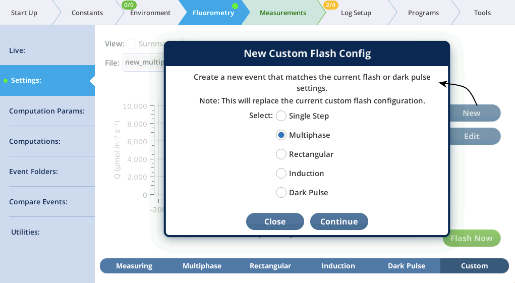
Figure 8‑66. Make a new custom flash event that will match the current settings for the multiphase flash. -
The Settings > Custom screen provides a summary view (Figure 8‑67) of the current custom flash definition that was just loaded.
If the custom flash definition has any convenience variables (this one provides 4), they are listed on this screen. These variables allow a flash to be adjusted without having to edit the actual definition table. How many variables a flash might have is entirely up to the user.
-
To see the actual definition table, tap the Edit button.
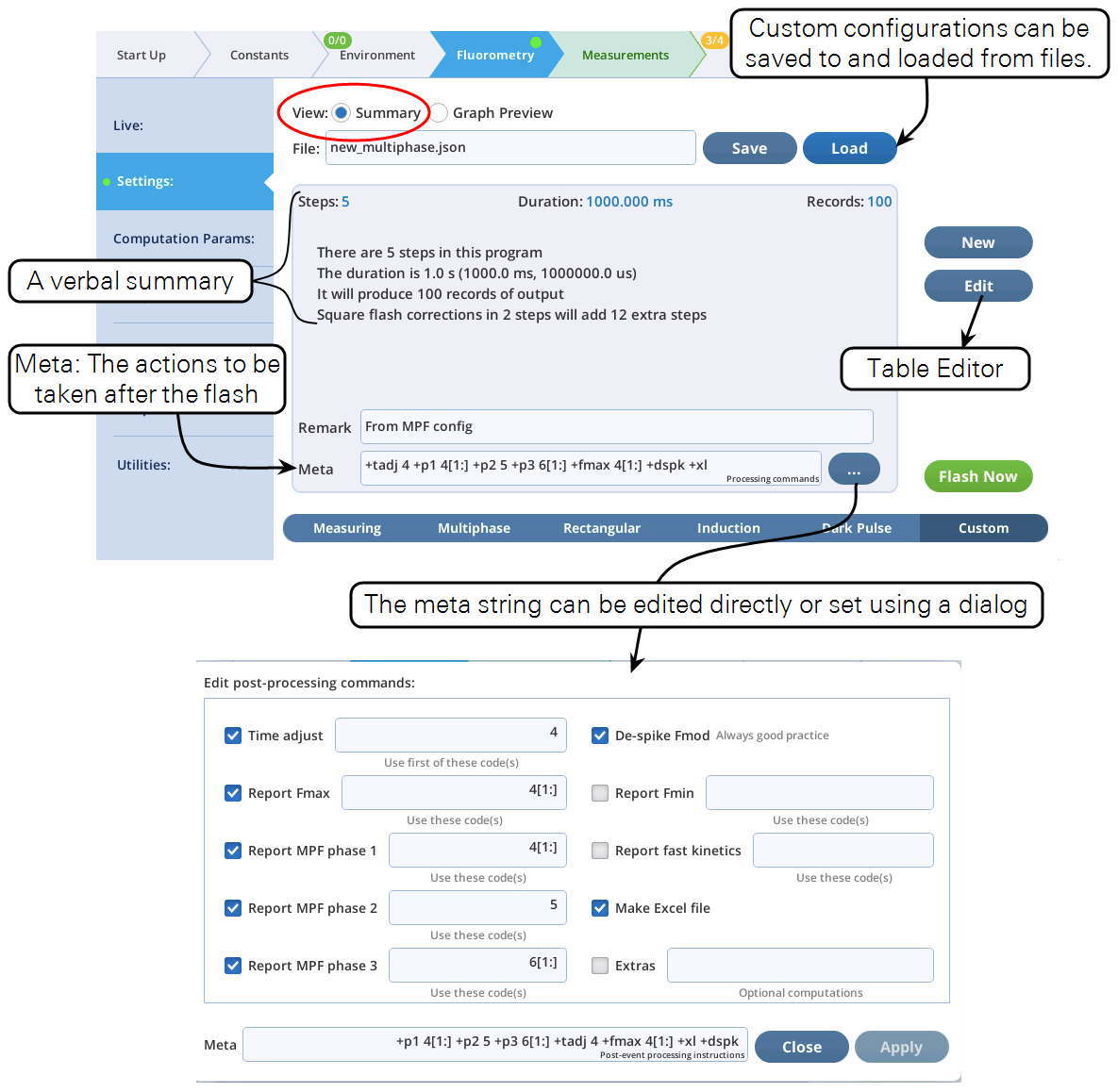
Figure 8‑67. The Summary view and Table Edit view of the custom flash generated by pressing the New button and selecting Multiphase. The complete table header has 10 columns, 9 of which specify what will happen for each step (row) of the flash. The #Pts column is there for your own information, showing results computed from the timing columns to its left.

-
Let's try making some edits to demonstrate how the Table Editor works.
First, select Cells to enter Cell edit mode. To edit a cell, tap it to select (highlight it), then tap Edit cell. The sequence below makes a series of changes in row 2 and illustrates the interactions between the timing columns.
The table editor has built-in relationships between the three timing-related controls.
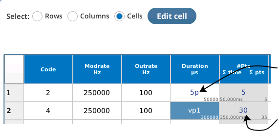
When an input cell has more than one value, the middle value is what is entered. The lower right value is what will be used. Example: 5p is a shortcut: It means pick a duration that will yield 5 data points, That duration, based on output rate, is 50,000 µs. The #Pts column is information only; it shows the number of output points this step (center), cumulative time (lower left), and cumulative data points (lower right). -
Change
Durationto '100000'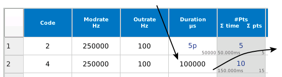
No lower right value, since it is the same as the entry. The shortened duration drops the output records to 10. -
Change
Durationto '0.12345s'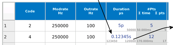
Now there are three duration values: the entry evaluations to 123456 µs (lower left), which leaves dead time (because of the 100 Hz output rate), so it will actually use 120000 µs (lower right) and yield 12 data output records. -
Change
Outrateto '1000'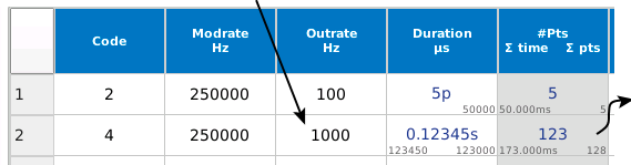
With the higher output rate, the effective duration is now 123000 µs (lower right), and yields 123 output records. -
Change
Outrateto '34500'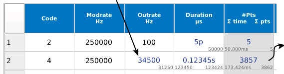
34500 is not an allowed output rate for a 250kHz modulation rate; it will use 31250 instead. Now the effective duration is 123424 µs, yielding 3857 output records. -
Change
Modrateto '55555'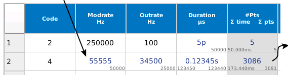
55555 is not an acceptable modrate, but 50000 is. This changes the allowable output rates, and 25000 is now closest to what we asked for. Effective duration is now 123440 µs, yielding 3086 output records.
-
-
Undo all these changes by tapping the Close button.
-
To see a graph of what the flash looks like, select Graph Preview (Figure 8‑68).
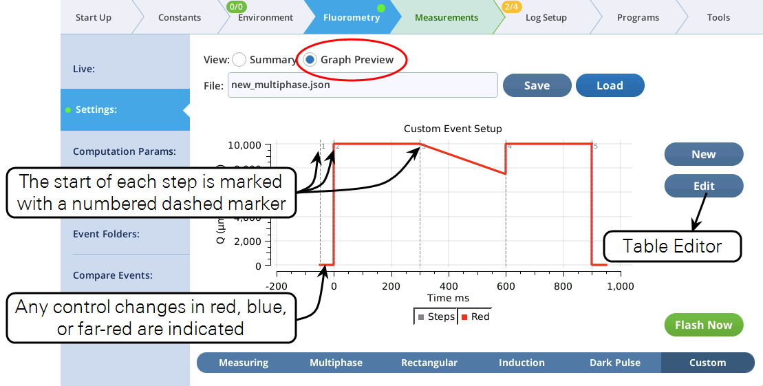
Figure 8‑68. The Graphical view of a custom event shows the start time of each step and any actinic light changes. -
Now let's modify this event by adding a OJ pulse (a 2 ms maximum intensity flash to measure the initial rise dynamics) right at the start (after the margin).
Go to the Table view, be sure you are in Row edit mode, tap row 5 to select it, then tap Insert (Figure 8‑69).
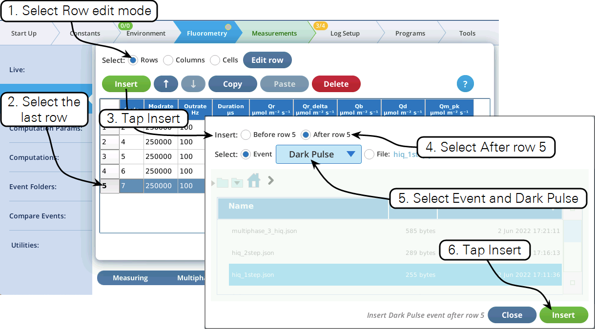
Figure 8‑69. Inserting an OJ pulse at the start of the event. -
Figure 8‑70 shows what the MPF config now looks like, with the OJ pulse inserted at row 2.
Tap Apply to keep the changes you made.
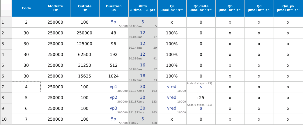
Figure 8‑70. The MPF flash with an OJ Pulse at the start. -
The graphical preview shows a combined MPF and dark pulse event (Figure 8‑71).
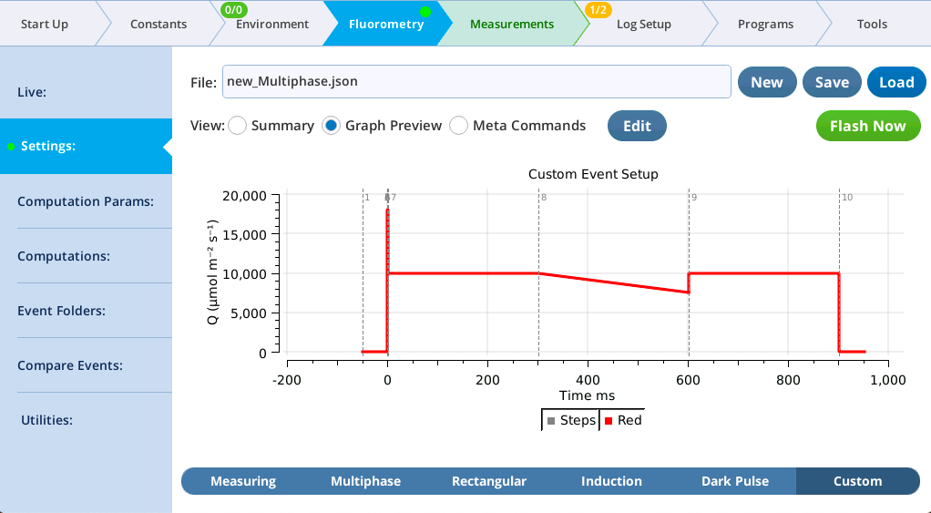
Figure 8‑71. Preview of the custom MPF with OJ pulse at the start. -
Test the custom event by tapping Flash Now and examining the results in the Compare Events screen (Figure 8‑72).
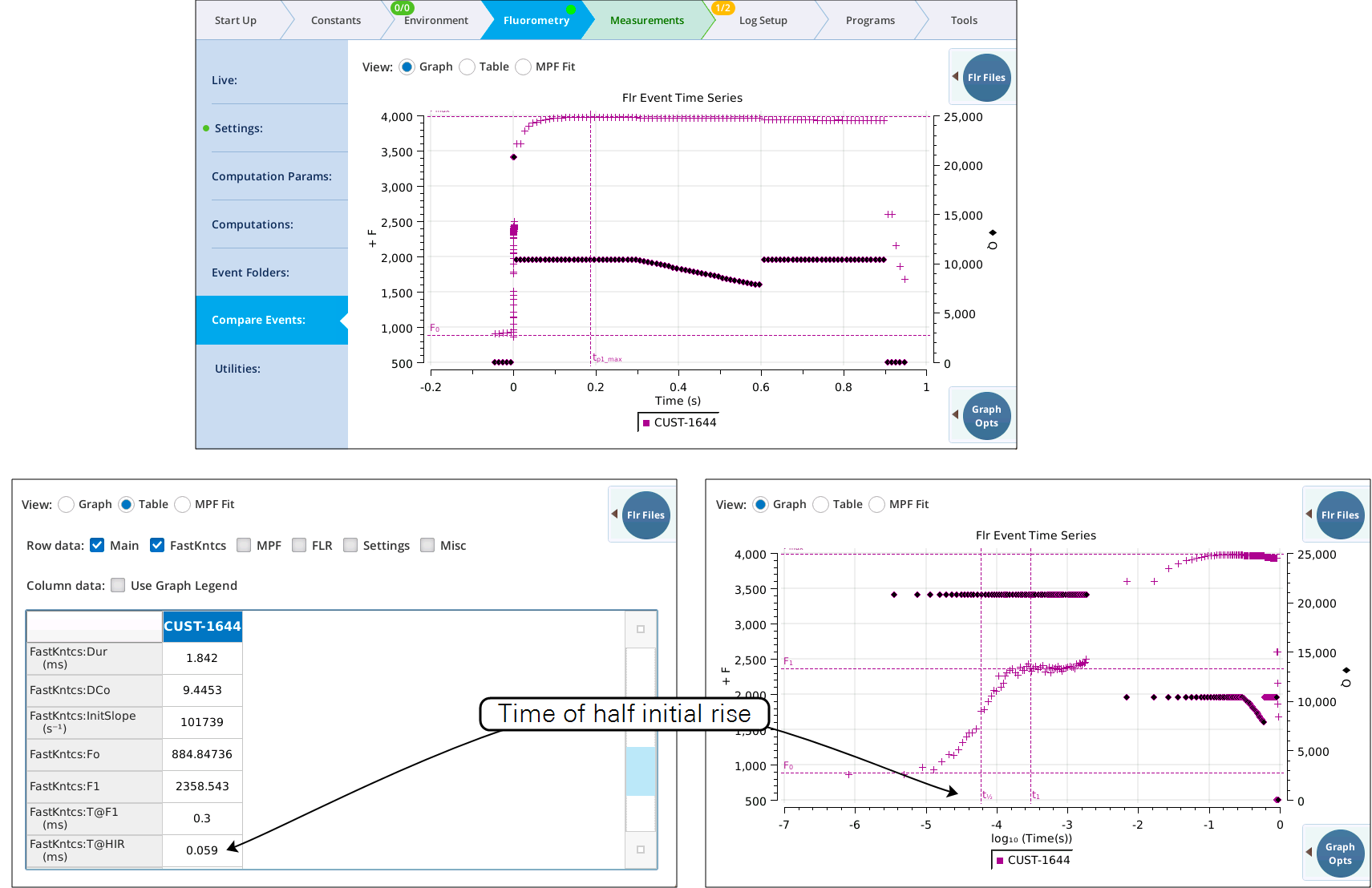
Figure 8‑72. The custom event results. The OJ pulse is evident with the log scale enabled (right), and the half-rise time listed in the fast kinetics section of the table (left). -
Save this flash definition by tapping in the file name edit box (Figure 8‑73) and entering an appropriate file name.
If you pick a name that already exists, you will be notified and given the choice of overwriting it or changing the name.

Custom event definition files
Save and load
The Settings > Custom screen provides file access for saving and loading custom events (Figure 8‑74).

All files are saved in the directory /home/licor/flr/custom. You can create subdirectories simply by adding them to the name you enter. For example, if you enter
bob/test/sample.json
the directories bob and test will be created (if they don't already exist).
Note that you are restricted to /home/licor/flr/custom.
If, for example, you attempt to save to the logs directory, by entering:
/home/licor/logs/sample.json
the resulting file will be here:
/home/licor/flr/custom/home/licor/logs/sample.json
The files are .json files. The .json suffix is automatically appended if you do not provide it.
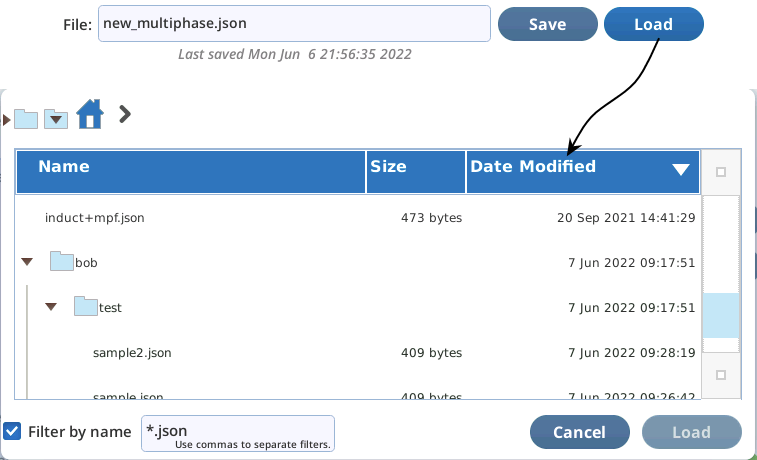
To read a saved file, tap Load. A file viewer dialog is provided for picking the file (Figure 8‑75).
File structure
A custom event definition file has two possible formats: the original format is illustrated in Listing 8‑1. Files created in version 2.2 and above are shown in Listing 8‑2. The original structure matches what is sent to the fluorometer to define a custom flash. The structure is a map of strings. With the exception of the meta and remark items, each string contains space-delimited values of the specified element for each step of the event. Note that some of the items, such as modrate, have only one value. The official number of steps is determined by the number of items in the duration string. When any other field is "short", the last item in that string is assumed to apply at all remaining steps.
Listing 8‑1. Original format of a custom induction flash file. Values of x mean to use that parameter's value prior to the event.
{
"meta": "+tadj 3 +fmax 3 +fk 3 +xl +dspk",
"code": "2 3 3 3 3 3 3 3 3 3 3 3 7",
"duration": "20.0 48 96 192 512 1024 1920 5120 9600 19200 48000 914288 40000.0",
"modrate": "250000",
"outrate": "250000 250000 125000 62500 31250 15625 6250 3125 1250 625 250 125 125",
"Q_red_setpoint": "x 15000 15000 15000 15000 15000 15000 15000 15000 15000 15000 15000 x",
"Q_red_delta": "0 0 0 0 0 0 0 0 0 s s s 0",
"Q_blue_setpoint": "x",
"Q_farred_setpoint": "x",
"Q_modred_setpoint": "x",
"remark": "From Induction config"
}
Listing 8‑2. Format starting in version 2.2. This example is a simple 3 step rectangular flash.
{
"version": 0,
"variables": [
{
"id": "#0",
"label": "vred",
"description": "Red target (add % for percent max)",
"value": "12000",
"count": 1,
"row": 0
},
{
"id": "#2",
"label": "vdur",
"description": "Flash duration (us. Options ms or s, t for total)",
"value": "1000ms",
"count": 1,
"row": 1
},
{
"id": "#1",
"label": "vmarg",
"description": "Margin time (or add p for points)",
"value": "5p",
"count": 2,
"row": 2
}
],
"meta": "+tadj 3 +fmax 3[1:] +dspk +xl",
"remark": "Rect_with_variables",
"def": [
[
"2",
"250000",
"100",
"vmarg",
"5",
"x",
"0",
"x",
"x",
"x"
],
[
"3",
"250000",
"100",
"vdur",
"100",
"vred",
"s",
"x",
"x",
"x"
],
[
"7",
"250000",
"100",
"vmarg",
"5",
"x",
"0",
"x",
"x",
"x"
]
]
}
Archiving and backup
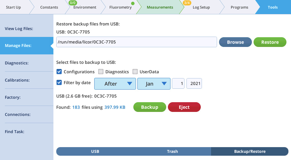
The /home/licor/flr directory is included as part of configuration in the LI-6800s backup facility (Figure 8‑76). The directory contains the custom folder (flash definitions), the extras folder (user defined meta computations), and the graphs folder (the Fluorometry > Compare Files graph saved settings).
The table editor
Custom flashes are built and modified largely through the Table Editor (Figure 8‑77). The table’s columns represent the various things that you can specify about the fluorometer’s state, such as red actinic intensity, modulation rate, etc. Each row of the table represents a time step. In the example below, the 5 steps make up an MPF flash: step 1 is a pre-flash “margin”, steps 2, 3, and 4 are the MPF phases, and step 5 is a post flash “margin”.
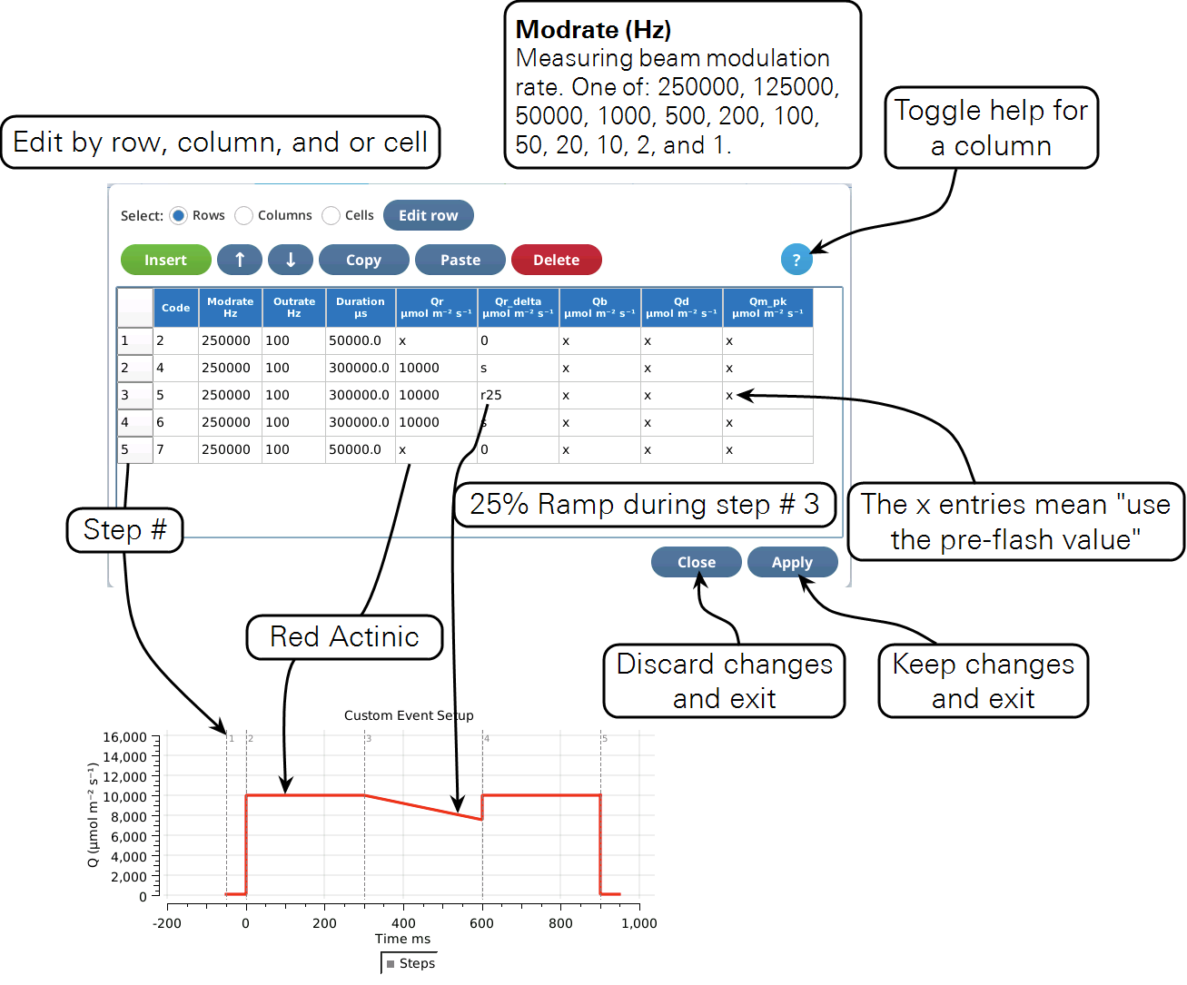
The table editor is a dialog; any changes you make are only retained if you tap Apply. To discard changes, tap Close.
Column help can be toggled on/off with the ? button.
When the Show Details box is checked, multiple values may appear in a cell (Figure 8‑78). For most cells, there are three possible values: the Entry value appears in the center, and is what the user entered (value, variable name, shortcut, etc.). At the lower left is the Evaluated value, which is simply what the variable or shortcut evaluates to. The Final value is at the lower right, and is what will actually be used.
When all three values differ, they are all displayed (left in Figure 8‑78). The Evaluated value is not displayed if it matches the Entry or the Final value (right in Figure 8‑78). If all three values match (or, if the Show details checkbox is unchecked), only the Entry value appears.

The #Pts column (Figure 8‑79) is unlike the other columns. It is there for your reference only as you configure a custom event. It shows for each step, the number of output records, the cumulative duration, and the cumulative number of output records.
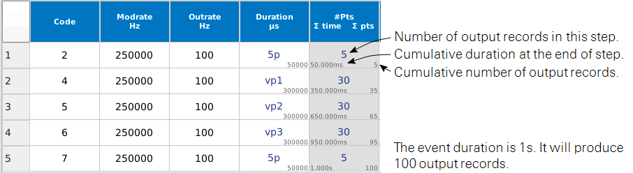
#Pts column shows status information and is not part of the flash definition.
Table 8‑12 provides a brief guide to each column in the Table view. For more details, see Custom event parameter reference.
| Label | Description | Entry Options1 | Units |
|---|---|---|---|
Code
|
The step identifier number. All records output during this step will carry this identifier. Code numbers are closely associated with the meta string that specifies post-event processing options, described in Meta commands. | numeric (2 .. 53) | |
Modrate
|
Measuring beam modulation frequency. | numeric2 | (Hz) |
Outrate
|
Data record output frequency. | numeric3 | (Hz) |
Duration
|
Duration of this step of the flash. | numeric4 | (µs) |
#Pts
|
Number points, cumulative duration, and cumulative points. | entries are ignored | |
Qr
|
The target intensity for the red actinic LEDs. | numeric | (µmol m-2 s-1) |
| Set to percent of full scale | n% | (n in %) | |
| Use the pre-flash value. | x | ||
Qr_delta
|
The amount to change (by linear ramp) the actinic LEDs during this step. | numeric | (µmol m-2 s-1) |
| MPF ramp percentage. See equation 8‑27. | rn | (n in %) | |
| Square flash correction code. See Qr_delta. | s or sn | (n in ms) | |
Qb
|
The target intensity for the blue actinic LEDs. | numeric | (µmol m-2 s-1) |
| Set to percent of full scale | n% | (n in %) | |
| Use the pre-flash value. | x | ||
Qd
|
The target intensity for the farred LEDs. | numeric | (µmol m-2 s-1) |
| Set to percent of full scale | n% | (n in %) | |
| Use the pre-flash value. | x | ||
Qm_peak
|
The target intensity for the modulating LEDs. | numeric | (µmol m-2 s-1) |
| Set to percent of full scale | n% | (n in %) | |
| Use the pre-flash value. | x | ||
Basic controls
Three editing modes are available: Row, Column, and Cell.
Row editing
Row editing operates on selected row(s) of the table. To select a row, simply tap it. Multiple selection is allowed (tap + drag).
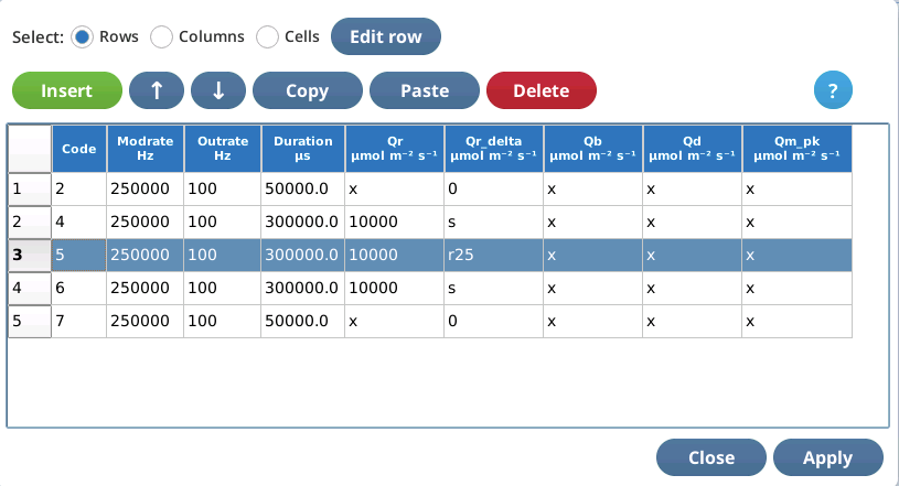
To edit a selected row (or first row of a multi-row selection), tap Edit row. The edit string consists of space-delimited values corresponding to the 10 Entry values of row. The 5th entry (30 in the figure below) belongs to the #Pts column; it doesn't matter what you enter for this, as this is always computed from the Duration and Outrate values.

If you enter more than 10 values, the extra values are ignored. If you enter less than 10 values, the missing ones remain unchanged.
Selected row(s) can be moved up or down with  .
.
The table editor has a clipboard that can contain one or more rows (and any associated variables). Selected rows are copied to the clipboard by Copy and inserted into the table with Paste, which inserts the clipboard contents before the selected row. If no rows are selected, Paste becomes Append, which appends the clipboard contents to the end of the file.
Note: the clipboard contents are maintained across visits to the table editor, allowing you to copy lines from one custom flash, and paste them into another. If the clipboard contains variables when pasted into a different event, the system will reuse clipboard variables if the name and values match; otherwise, a new, uniquely named variable is created in the destination.
Delete removes selected row(s) from the table.
Insert allows external custom flash steps to be inserted into the table above or below the first selected row (Figure 8‑81).
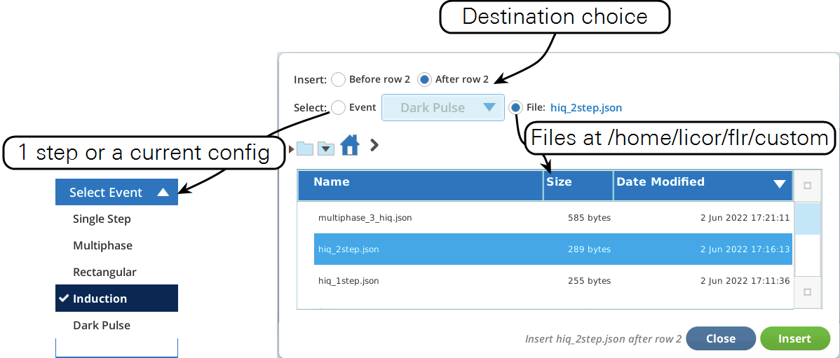
The standard insert options are
-
Single Step - Same as the step in the New dialog.
-
MPF (no margins) - Same as the Multiphase option in the New dialog, except without the margin steps.
-
Dark (no margins) - Same as the Dark Pulse option in the New dialog, except without the margin steps.
-
OJ Pulse - Essentially this is the first 1.8 ms of an induction curve, and supports the fast kinetic computations through F1.
-
OJIP Pulse - This is the first 88 ms of an induction curve, to support all of the fast kinetics computations.
-
HIQ Response - This is a 100 ms sequence that measures high intensity quenching (HIQ) response as a function of light intensity at 8 intensities, with two (50% and 100% intensity) repeated at the end as a repeatability check.
Column Editing
Column editing (Figure 8‑82) operates the currently selected column. Tap in a column to select it.
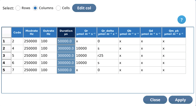
To edit the selected column, tap Edit col. The edit string consists of space-delimited values for that column for each row of the table.

If you enter too many entries, the extra ones are ignored. If you enter too few, the deficit is made up from the last value in the list. For example, to set an entire column to the same value, just enter one value when column editing.
Cell editing
Cell editing (Figure 8‑83) operates on the currently selected cell. Tap in a cell to select it.
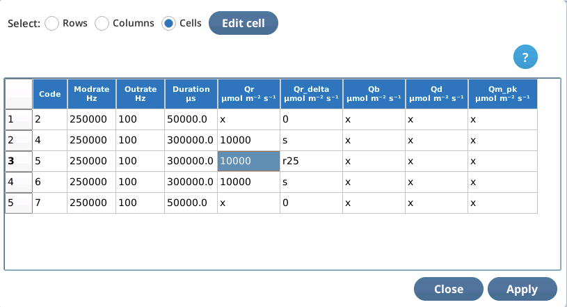
To edit a selected cell, tap Edit cell.

Shortcuts
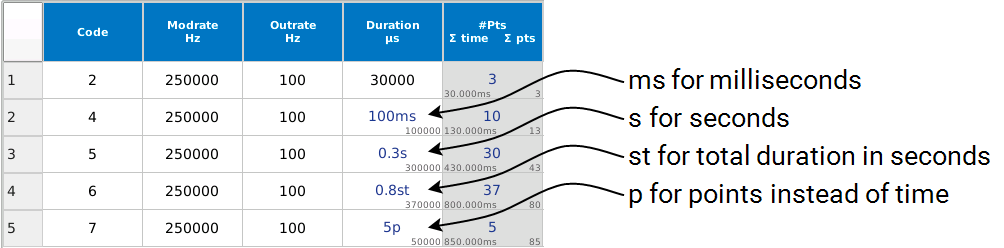
The Custom Flash Table Editor supports some shortcuts (see Table 8‑13) that simplify editing. Most are used only for duration cells. One is available for cells in other columns.
Some rules for using shortcuts:
tcan be used in combination with s or ms.pcannot be used with s, ms, or t.- Order or position do not matter. For example
100mst=t100ms=10t0ms=1ms0t0, etc. - Duration shortcuts can be used in Row, Column, or Cell edit mode (as long as it is used for the duration value). | can be used in any edit mode for any column.
- Variable values (see below) can include the duration shortcuts.
- All shortcuts except | are preserved in the Entry value (or variable value) for a cell. The | shortcut is not preserved and it does nothing if entered for a variable's value.
Figure 8‑84 demonstrates the Duration shortcuts.
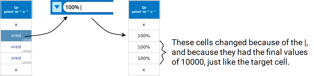
The | shortcut sets all cells having the same final value in a column with one edit. The original (pre-edit) Final value of the target cell is used, once that cell is edited, to find all the other cells in that column with a matching final value, and sets them to the same new Entry value as the target. Figure 8‑85 demonstrates the | shortcut.
Variables
Variables (defined within the scope of a single custom flash definition) make it easy to change a custom flash file's behavior without having to actually edit the table. Typical examples: a variable that determines the flash duration of one or more steps, or one that specifies the maximum red target. Variables can be used in any of the columns (except #Pts, where entries are ignored).
Variables can be created and edited from the Custom Flash Summary screen. They can also be created and set within the table editor. Variable names have one simple rule: they should start with a v (or V). To add a variable, edit the cell and enter the name.
If the variable does not yet exist, the default value will be whatever the current final value of the cell is. If you want to add a variable and set a value in one step (or change the value of an existing variable), enter the name, and value, separated by =.
Step-by-step example:
-
Press New in the Summary screen and select a Rectangular flash.
Then tap Edit to open the Table Editor.
-
Let's make a variable for Outrate.
In Cell edit mode, highlight the row 1 Outrate and tap Edit cell. Enter v1.

-
Now, edit row 2 Outrate. Make this v1, but also change the v1 value to 200.

-
Now, edit row 3 Outrate, setting it to v1.

-
Tap Accept to keep these changes, and return to the Summary screen, and note the presence of the new variable v1 in the list.
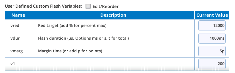
-
Check the Edit/Reorder box, and enter a description for v1.
Note you can also choose a more descriptive name. Let's call it
vout.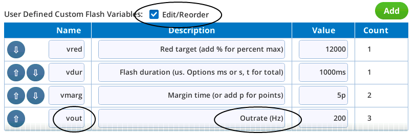
-
Just to be sure, tap Edit again and verify that v1 has been renamed.
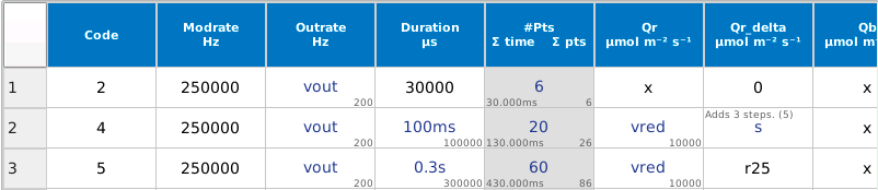
One final note: Steps 2, 3 and 4 could have been consolidated into a single step by making use of the * shortcut:

It could also have been done from Column edit mode, by entering a single entry, v1 = 200, which would be applied to all the missing rows/entries.
Following the rules
Custom Flash configuration parameters have a number of constraints, notably for the timing parameters (for details, see Custom event parameter reference), as well as limits on the number of steps, total time, etc. The Custom Flash Table Editor knows the rules, so you don't have to, as the following examples illustrate:
-
Permissible values. Several custom flash settings have a restricted range of possible values. If a requested value is in fact not allowed, or (for duration) inefficient, the cell will show the value it is going to use in the lower right corner (the Final value).
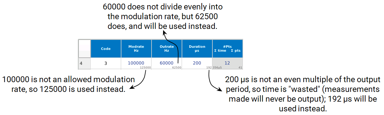
Figure 8‑86. Cells in the Table Editor show what you asked for, and what you will get (if it differs). -
Step limits. A custom flash can consist of no more than 38 steps (i.e. rows in the table). Square flash corrections (see Qr_delta) will reduce the available number of steps.
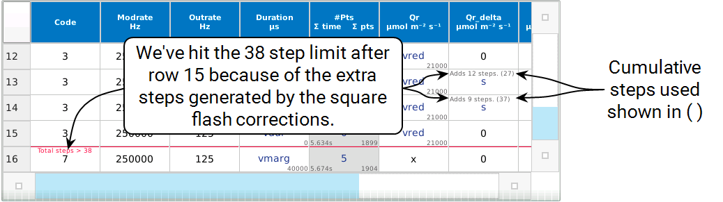
Figure 8‑87. The Table Editor will warn about too many steps, and why. -
Time limits. The sum of the Duration items can be no greater than 10 seconds. A single step's
Durationhas the same limit.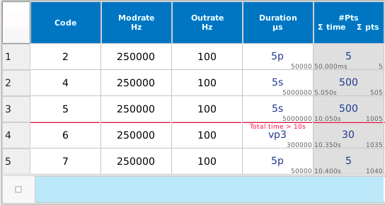
Figure 8‑88. The Table Editor is showing the time warning because of the two long durations in steps 2 and 3. -
Data limits. The total number of data records output for a flash cannot exceed 20,000 (the practical limit is much lower - see below). The number of output records ni for the ith step can be computed from the output rate (Hz) and the duration (s):
8‑25
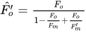
and the summation of output records over all N steps must satisfy
8‑26

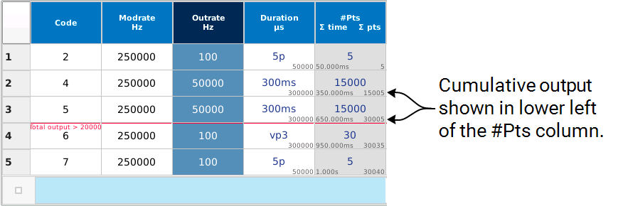
Figure 8‑89. The Table Editor is showing the output warning because of the high output rates and long durations in steps 2 and 3.
Note: The larger the number of output records, the longer the whole process (data transfer to the console and processing on the console) will take. As a practical limit for reasonable processing times, consider keeping the total number of records below 5,000. As an example, a 5,000 record induction curve will take about 20 seconds to acquire, and another 15 seconds to plot on a console with a 4-CPU digital board. On the older 1-CPU board, it will take about 6 times longer.
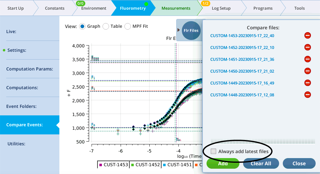
If you really need that much data, then disable automatic plotting by clearing the Always add latest files checkbox on the Compare Events screen's Flr Files pullout dialog (Figure 8‑90).