Examples and Procedures

This chapter contains step-by-step instructions for most of the common operations with the LAI-2200C and FV2200.

Each Example tells how to measure LAI with a particular optical sensor (wand) configuration or canopy type. Examples 2, 4, and 5 include the scattering correction for use with direct sun conditions. When using two or more optical sensors with scattering correction, see Multiple Sensors With Scattering Correction.

Each Procedure describes a particular task on the console or in post-processing. These procedures are referenced from various locations in this manual.

Example 1 - One Sensor Measurement without scattering correction

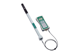
This step-by-step section requires one LAI‑2270C Control Unit and one LAI‑2250 Optical Sensor and view caps. Follow these steps:

1. Place the desired view cap on the sensor with the opening pointing away from the handle. Attach the optical sensor to the control unit (either the X or Y terminal) and turn on the control unit. Verify that the sensor is operating correctly by placing a hand over the lens and observing that the reading drops (in Monitor Mode). Remove your hand and notice that the reading returns to normal.
2. Set prompts, if desired.
3. Open a file (Procedure 2.2 - Opening a New Data File). Enter responses to the prompts and press OK to save or EXIT to skip the prompts. Now the LAI-2200C will enter Logging Mode and is ready to record data.
4. Position the optical sensor above the canopy. Be sure it is level and that no foreign objects are in view of the sensor. Verify that the ABOVE LED is illuminated (press the A/B button on the wand if it is not). Press the LOG button on the wand or control unit to record an Above reading.
5. Press the A/B button (the ABOVE LED will turn off). Hold the optical sensor below the canopy(level and oriented in the same direction as the above-canopy reading was) and press the LOG button to record a Below reading.
6. LAI, MTA, SEL, and SEM values will be visible in Logging Mode (use the arrow keys to change what is displayed).
7. Continue making B readings, moving the sensor to a new location each time. Typically, the distance between B readings is on the order of the canopy height. You can intersperse A readings as necessary, if sky conditions or the view direction changes.
8. When you are finished, press the START|STOP button to close the file and exit Logging Mode.

Example 2 - One Sensor Measurement with Scattering Correction

This example is of an LAI measurement that would normally be made by doing an A reading, followed by a series of B readings. Thus, our sequence (if we weren’t doing scattering corrections) might be ABBBB. Because we are doing scattering corrections, we will want to replace the A readings with a 4A sequence. Thus, we’ll end up with a record sequence of AAAABBBB.

Preliminary steps are just like the previous example.

1. Perform a 4A sequence (Procedure 2.6 - Logging a 4A or 3A Sequence).
2. Log the B readings.
3. Close the file (press START|STOP).
4. Transfer the file to FV2200 (Procedure 3.1 - Moving Data to a Computer).
5. Convert the 3A or 4A sequences to K records (Procedure 3.9 - Generating K records from Sequences).
6. Enter the remaining scattering inputs (step 6 of Procedure 3.11 - Set Scattering Inputs for a Group of Files).

Note: For more details about measurements with scattering correction, see Protocol Suggestions for Direct Sun.

Note: When using two or more sensors with scattering correction, see Multiple Sensors With Scattering Correction.

Example 3 - Two Sensor Measurement without scattering correction

The Match Methods mentioned below are discussed in Three Methods for FV2200 Matching.

1. Place the desired view caps (same size) over the lenses of two optical sensors (see chapters 4 and 6). Connect the optical sensor to the control unit and turn on the control unit.
2. Synchronize clocks in both wands (Procedure 1.4 - Synchronizing Wand and Console Clock), and delete any data from the above wand (MENU > Data > Wand > Purge).
3. Start the Above wand autologging (Procedure 2.7 - Automatic Logging - Wand).
4. Disconnect the Above wand, and place it in an area that affords a clear view of the sky. Be sure it is level, stable, and oriented so that it views the same sky as the below canopy sensor will see.
5. Before leaving the A unit:
   1. If you are doing Match Method 2, create your match file now (Procedure 2.5 - Creating a Match File for Match Method 2).
   2. If you are doing Match Method 3, record your match data by opening a file and logging a few A readings with the sensors together. Leave the file open for the B records.
6. Go to the site for measuring B records, and record the readings. For each one, make sure it is seeing the same sky as the A unit.
7. (Match Method 3 only, optional) Before closing the file, return to the A unit, and append 1 or 2 A readings into the file.
8. Press START|STOP to close the file.
9. If you are doing Match Method 1 or 2, repeat step 6 as necessary, creating more below files. If you are doing Match Method 3, then you have to repeat steps 5 through 8 as needed.
10. When you are done, disable autologging on the above sensor (Procedure 2.7 - Automatic Logging - Wand) and download the files from the sensor to the control unit (Procedure 2.13 - Moving Wand Data to the Console).
11. Move the above and below files onto your computer (Procedure 3.1 - Moving Data to a Computer).
12. Import A records from the above file into the below files (Procedure 3.8 - Import A and Adjust A Records - FV2200).

Note: When using two or more sensors with scattering correction, see Multiple Sensors With Scattering Correction.

Example 4 - Forest Sites with One Sensor (and Control Unit)

This method is best suited to a clear blue day. The strategy is to start at a clearing and make A and K readings in an “above” file. Then move to the measurement site and measure each transect or plot in separate "below" files. Finally, return to the clearing and make final A and K readings. FV2200 is used to put everything together, do the scattering corrections, and compute final results.

1. At the A site, open a file (Procedure 2.2 - Opening a New Data File). We’ll assume the name is “above”, and log a 4A or 3A sequence (depending on the size of the clearing) (Procedure 2.6 - Logging a 4A or 3A Sequence). Close the file.
2. Measure each transect or plot into a separate below file. Each will have any number of B records.
3. Return to the A site, and repeat step 1, open file “above” and append another 4A sequence into it. Close the file.
4. Read all files into FV2200 (Procedure 3.3 - Loading Data Files into FV2200). They can all be in one view.
5. Generate K records in file “above” (Procedure 3.9 - Generating K records from Sequences).
6. Import K records to the below files (Procedure 3.12 - Combining Multiple Files - FV2200).
7. Import A records to the "below" files (Procedure 3.8 - Import A and Adjust A Records - FV2200). Enable interpolation, and don’t do adjustments (since A and B are the same sensor).
8. Set the rest of the scattering inputs on the "below" files (step 6 of Procedure 3.11 - Set Scattering Inputs for a Group of Files).

Example 5 - Forest Sites with One Sensor (without Control Unit)

The only difference between this example and the one above is that we don’t have separate files; everything gets collected by the wand and winds up in one file. Again, this is best on a clear blue day.

1. At the A site, log a 4A or 3A sequence (depending on the size of the clearing).
2. Move to measurement sites, and log B records. You will need to mark the start of each new ‘file’: you could log a fake A record, or cover the lens with your hand and log a record with tiny values in it. Later on, you will use these markers and eventually delete them.
3. Return to the A site, and repeat step 1.
4. Copy the wand data to a control unit (Procedure 2.13 - Moving Wand Data to the Console). We'll call this file ‘BIG’, since it is the big file from which we’ll make the other files, one for each transect or plot.
5. Load ‘BIG’ into FV2200 (Procedure 3.3 - Loading Data Files into FV2200).
6. Generate K records in ‘BIG’ (Procedure 3.9 - Generating K records from Sequences).
7. Set the rest of the scattering inputs in ‘BIG’ (step 6 of Procedure 3.11 - Set Scattering Inputs for a Group of Files).
8. In the main view of FV2200, copy ‘BIG’ (highlight it and hit copy button (or File > Copy). Then paste (File > Paste) as many copies into that same view as you have transects or plots.
9. For each file pasted, double click it to get the detail view and do the following:
10. 
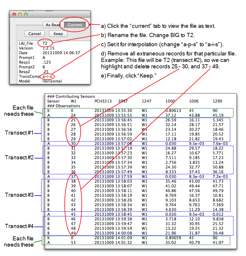
10. Click the Keep button.

Example 6 - A Simple Isolated Canopy

Consider the example given in A Simple Example. In this example, the plant is a hemispherical shrub with measured path lengths of 0.7 m. Launch the FV2200 software. Click on File > Sample files > Manual Examples.txt. Double click on the file called SHRUB to view file details, then select the As Read tab. The data file for this shrub looks something like this:

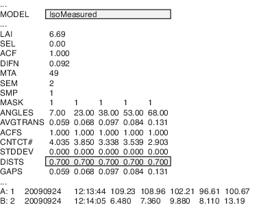
The LAI value is foliage density. There are two ways to tell this by looking at the file. One is the MODEL line. “Horizontal” means the canopy model is horizontally infinite, or at least large enough that the default DISTS vectors apply. “IsoMeasured” means an isolated canopy. The other way to know this is to look at the DISTS values. Since they are not the default values (1.008, 1.086, 1.269, 1.662, and 2.669), then LAI should be interpreted as foliage density.

Click on the Header tab, then click Change. In the Recompute dialog, check Change Canopy Model, then check Change View Cap. Select the 90 degree cap and observe changes in the Volume and Area fields, which are used to compute Drip Line LAI (DLLAI).

Example 7 - Isolated Tree

Below is an example of the procedure that could be used to measure LAI for an isolated plant. The steps below will generate a file much like the example file named TREE1 in the FV2200 software, which is accessed by going to File > Sample files > Manual Examples.

1. Create a new file with default Transcomp settings. Use a 90° view cap and take one AB pair in each of the four directions.
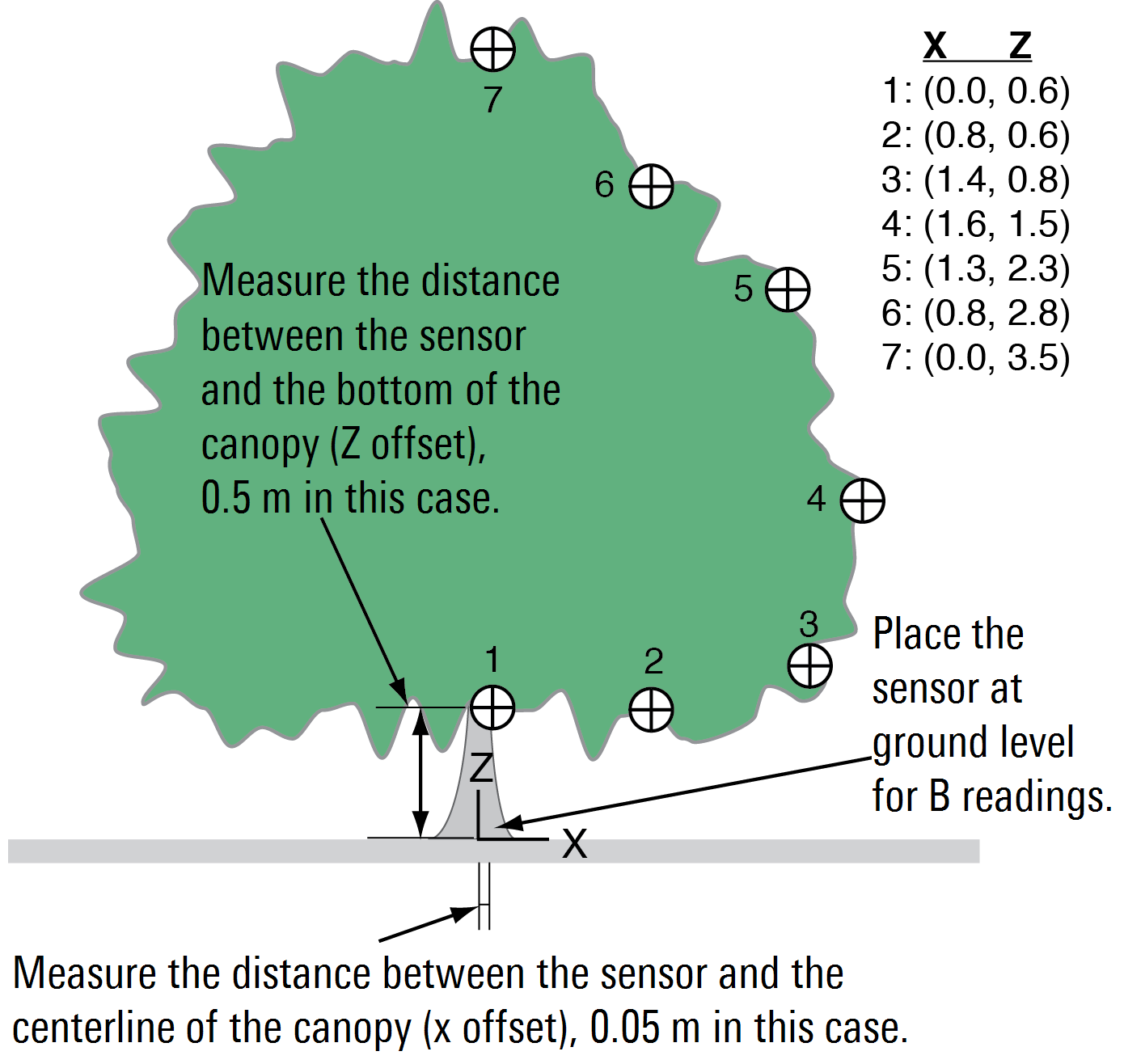
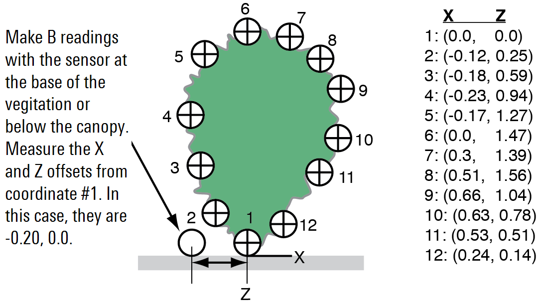
2. Measure the average shape of the tree’s crown with several X, Z pairs of points that describe the profile, as shown below (a photo of the profile with a meter stick for scale could be used as well).
3. Measure the X and Z offsets, as shown below.
4. 
4. Open the file with the FV2200 software.
5. Select the file and click the Recompute button. Check the Change Canopy Model box.
6. Check the Isolated Computed box, and the Change vertical profile box.
7. Click the Edit… button and enter the X, Z coordinates to define the canopy shape. Right click on the profile to add more points. Click OK when finished.
8. Enter the X and Z sensor position. Observe changes in volume and area values as these fields are updated.
9. 
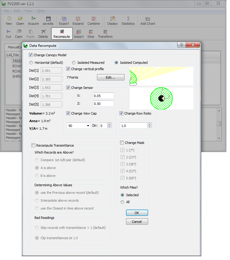
9. Click OK to implement the changes. The new LAI value, along with a summary of the procedure, will be visible in the log.
10. Save the file to retain any changes.

Example 8 - Isolated Row 1

There are two approaches that can be used to measure an isolated row, such as a grape vine or hedge. The first is described here, and the second is described for "Row 2" below.

The steps below will generate a file much like the example named ROW1 in the FV2200 software, which is opened by clicking on File > Sample files > Manual Examples.

1. Set the console Transcomp settings to Define Above: A; Determine Above: Interpolate; Bad Readings: Clip. Place a view cap with a 90° opening over the lens and create a new file.
2. 
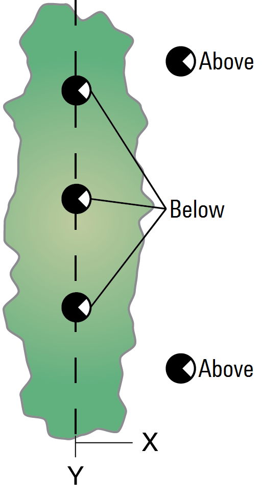
2. Make an above-canopy reading, multiple below-canopy readings, and a second above-canopy reading. Make the below canopy readings with the sensor at the base of the canopy, as shown.
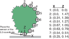
3. Measure several X, Z coordinates (meters) to characterize the vertical profile, perpendicular to the centerline of the hedge. This example uses 8 coordinates. See the following figure.
4. 
4. Measure the width (Y) and depth (X) of the hedge to compute the row ratio (Y/X), 5 in this case.
5. Open the data file in the FV2200 software.
6. Click the Recompute button. In the Recompute Dialog box, select Change Mask. Deselect ring 5 because it did not “view” any foliage.
7. Next, check the Change Canopy Model check box, then the Isolated Computed radio button. Check the Change Vertical Profile button, then select Edit….
8. Enter the X, Z coordinates to define the shape of the hedge. Right click on the canopy profile to add more points.
9. Check the Change Row Ratio box and set the row ratio to 5. Click OK.
10. 
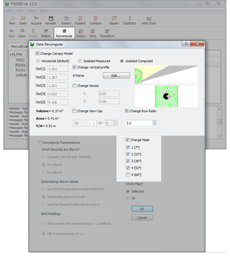
10. The new LAI values are displayed in the Log. Save the file to retain changes.

If the hedge were asymmetrical, two files would be required, one for each side of the canopy (or row 2 below could be used).

Example 9 - Isolated Row 2

The steps below will create a file similar to the example ROW2 in the FV2200 software, which is opened by File > Sample files > Manual Examples.

1. Set the console Transcomp settings to Define Above: A; Determine Above: Interpolate; Bad Readings: Clip. Place a view cap with a 90° opening over the lens and create a new file.
2. 
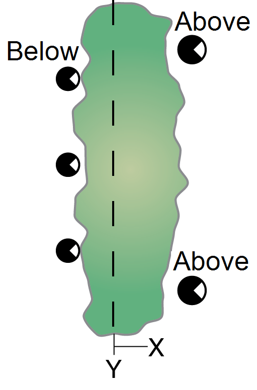
2. Make an above-canopy reading, several below canopy readings, and a final above-canopy reading. Take the below-canopy readings along a line that is parallel to the centerline of the shrub, but not directly under the shrub, as shown.
3. Measure a number of X, Z coordinates (meters) to characterize the vertical profile, perpendicular to the centerline, of the hedge. Measure the distance between where the B readings were taken and the centerline of the hedge (X offset), -0.20 in this case, and the distance between the vegetation and the sensor (Z offset) in meters (0.0 in this case), as shown in the following figure.
4. 
4. Measure the width (Y) and depth (X) of the hedge to compute the row ratio (Y/X).
5. Open the data file in the FV2200 software.
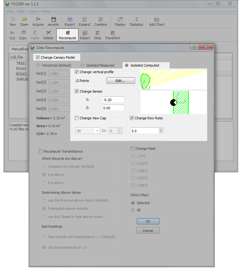
6. Click the Recompute button. In the Recompute Dialog box, check the Change Canopy Model check box, then the Isolated Computed radio button. Check the Change vertical profile button, then select Edit….
7. Enter the X, Z coordinates to define the shape of the hedge. Right click on the canopy profile to add more points.
8. Check the Change Sensor check box.
9. Check the Change Row Ratio box and set the ratio. Click OK.

The new LAI value is shown in the Log. Save the file to retain changes.