Example: Measuring the light response

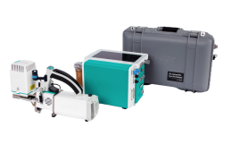
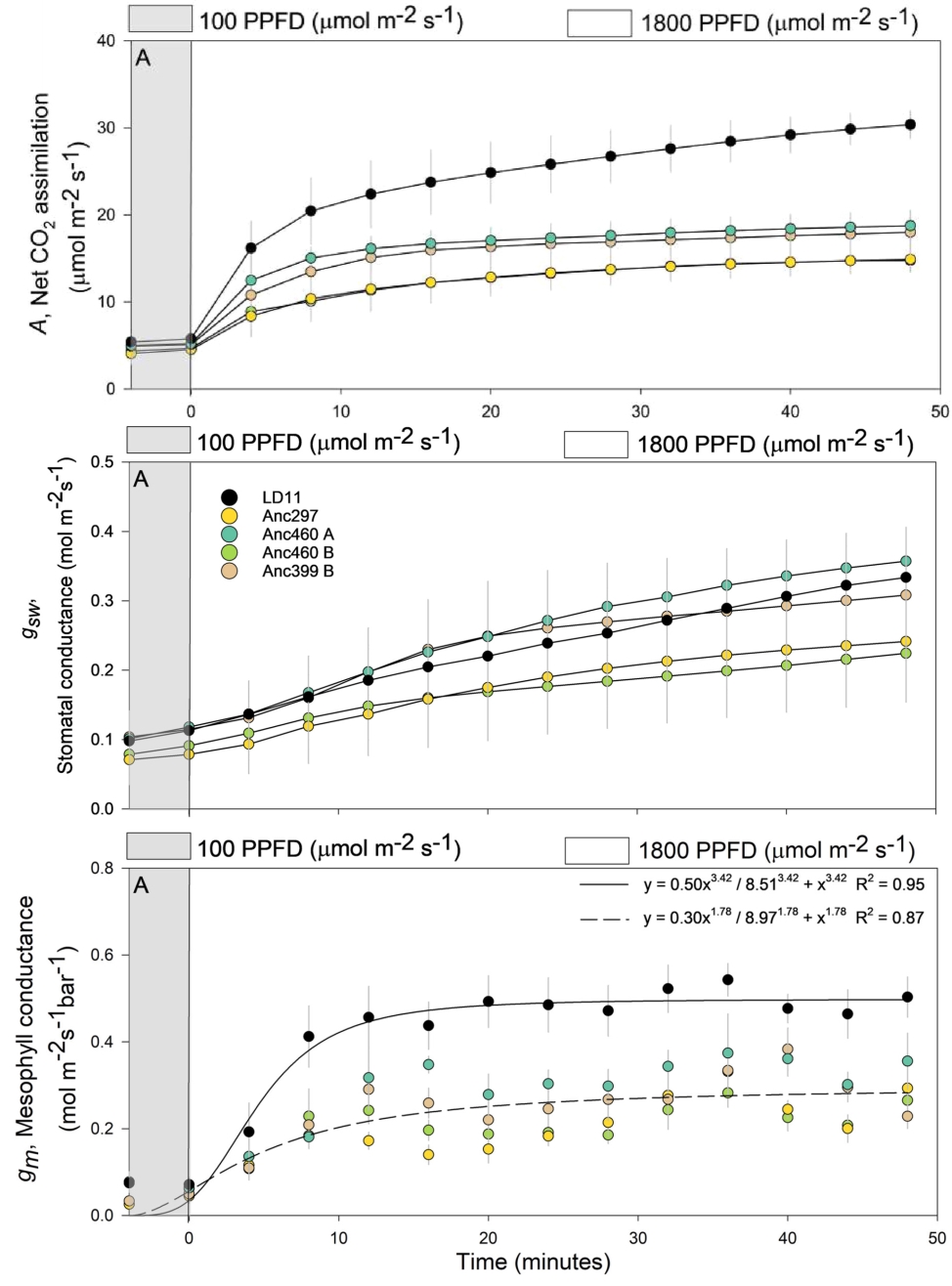
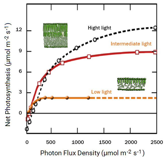
This section provides an example protocol for measuring steady-state A-Q with an LI-7825 gas analyzer. The aim of this experiment is to discover the light effects on A, g_sw and g_m (see Figure 12‑54). The light response curve should begin at low light and proceed to high light and time must be given at each light level for light acclimation. Typically, g_sw is the slowest to acclimate, requiring 20 to 60 minutes at each light level.

1. First, go through the suggested warmup procedure (Suggested warmup procedure).

   This process can take more than an hour, so be patient.

2. (Optional but recommended) After running the LI-6800 warm-up tests (Step 3), do a TGA zero and optionally, a 1-point span if span gas is available.

3. After calibrating the TGA, proceed to step 4 in Suggested warmup procedure, to do an isotopic calibration (after reaching a suitably low H₂O concentration in the TGA flow path). See Isotopic calibrations.

4. Check Constants > Gas Exchange.

   • Set leaf area if the leaf is not filling chamber.
   • Check stomatal ratio setting. Confirm the setting is correct for your leaf.

5. Check Constants > Leaf Light.

   Check the absorptance constants being used for each color of the light source installed is appropriate for your species.

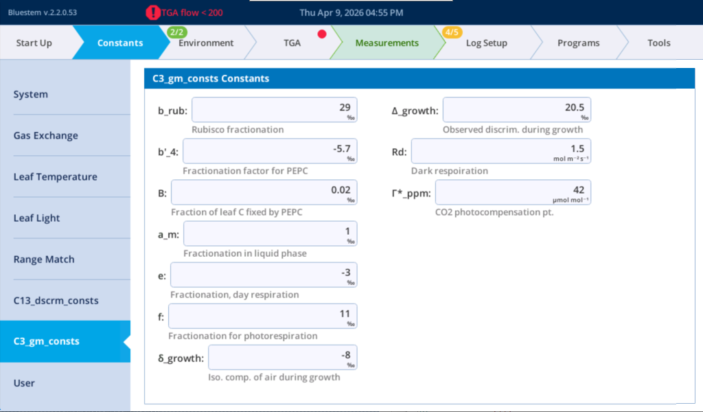
6. Check C13_discrim_consts and C3_gm_consts.

   Use defaults, unless you have a better setting.

   

7. Set Environment > Flow.

   • For 6×6 chamber: Set flow to 1,000 µmol s^-1.
   • For 3×3 chamber: Set flow to 600 µmol s^-1.
   • For 6 cm2 fluorometer: Set pump speed to medium and flow to 300 µmol s^-1.

8. Set Environment > H2O.

   Control VPD_leaf between 1 and 1.5 kPa.

9. Set Environment > CO2.

   Control CO2_s at 420 µmol mol^-1.

10. Set Environment > Fan.

    Control at 10,000 rpm.

11. Set Environment > Temperature.

    Control Txchg at 25 °C (or ambient temperature).

12. Set Environment > Light.

    • The light settings will be controlled during experiment, but off at the beginning.
    • Set color spec to 10% blue.
    • For the fluorometer, limit blue to 40 µmol m^-2 s^-1.

    

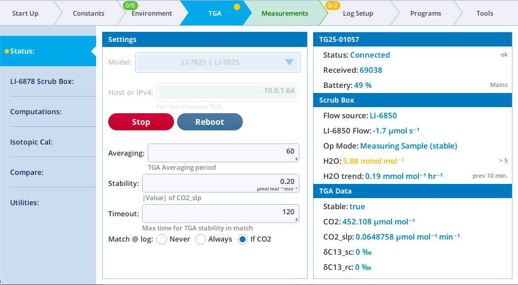
13. Set TGA > Status > Settings.

    • Averaging: Use 60 to 120 seconds.
    • Stability: Use 0.2 to 0.3 µmol mol^-1 min^-1.
    • Timeout: Set for 2x the averaging time; e.g., 120 to 240 seconds.

    

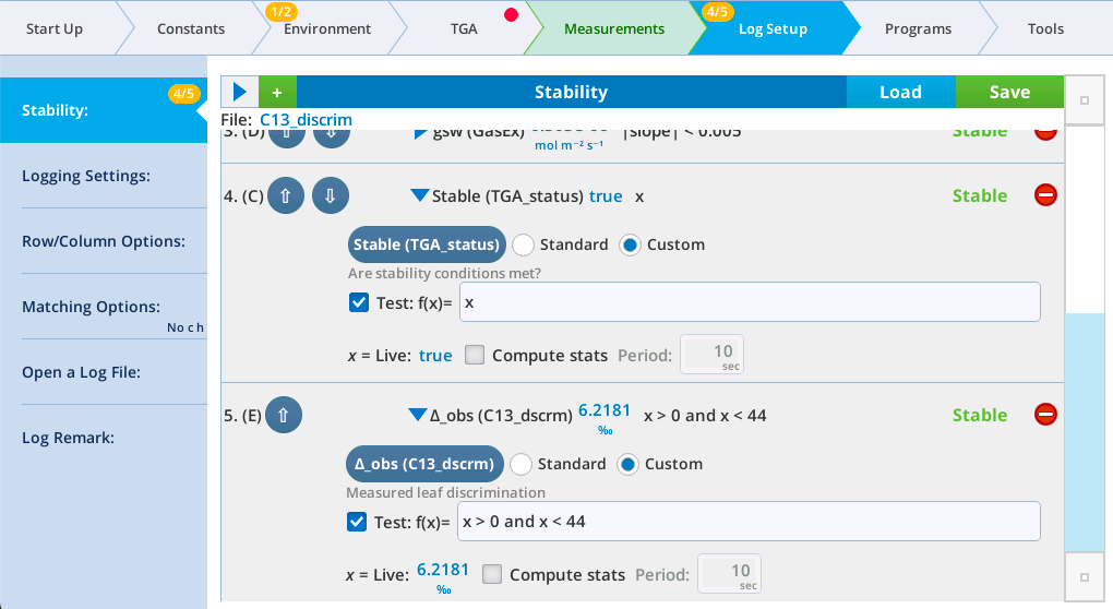
14. Set Log Setup > Stability.

    Tap Load and select the file named C13_discrim. It checks for TGA stability as you’ve defined it, and also that ∆_obs is a reasonable value. (No statistics on ∆_obs, since it is already an averaged TGA-derived value.)

    • ΔCO2: Period 20 seconds, slope limit 0.5 µmol mol^-1 min^-1.
    • ΔH2O: Period 20 seconds, slope limit 0.05 mmol mol^-1 min^-1.
    • gsw: Period 20 seconds, slope limit 0.005 mol m^-2 min^-1.
    • Stable (TGA_status): Custom, Test: f(x) = x.
    • Δ_obs (C13_dscrm): Custom, Test: f(x,m,s,d) = x > 0 and x < 44, compute stats period 30 seconds.

    

15. Set Log Setup > Row/Column Options.

    • Make sure the C13_dscrm_consts and C3_gm_consts are all checked to log as a row.
    • Include TGA_stats and any other optional groups you wish.

16. Set Log Setup > Matching Options.

    • CO2 match: Only match If Time > 10 mins since last match.
    • H2O match: Only match if Time > 10 mins since last match.

17. Open a Log File.

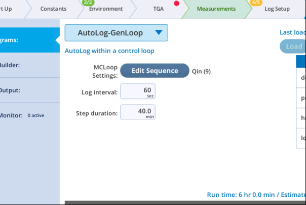
    • Set Programs > Programs > AutoLog-GenLoop.
    • Edit Sequence to parameter Light:Qin and set the light level sequence you wish. Use 0, 50, 100, 300, 600, 1000, 1500 µmol m^-2 s^-1. If using a field-grown plant, add an extra point at 2,000.
    • Log interval 60 s.

    

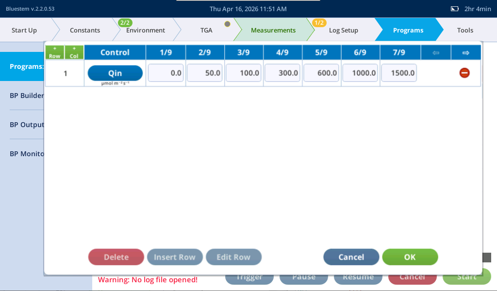
    • Step duration 40 min (this may not be long enough for gsw but is a good starting point.)

    

18. Start the program.

19. Monitor the Measurements tab.

    If you haven’t already configured grid and graphs for the TGA, load the example file TGA-25 (or TGA-25F if using the fluorometer). See Grid and graph settings for TGA Support. This will do the following:

    • Grid 4 is set with common TG25 related parameters and calculations.
    • Graph E shows real-time δC13 reference and sample values.
    • Graph F shows real-time observed, simple C3 model, and infinite gm discrimination values.
    • Graph G is setup with the A-Q curve, if the fluorometer is installed ETR is also shown.

20. Monitor Programs.

    The program progress is shown. After the program is complete, go to Log Setup > Logging to > and close the file. An *.xlsx file will be created on close

21. Download the files and analyze the data using your favorite software.

    A variety of modern tools are listed at Curve fitting tools.